De Casteljeau algorithm: The control points P₀, P₁, P₂ and P₃are combined with line segments termed as 'control polygon', even if they are not actually a polygon although rather a polygonal curve.

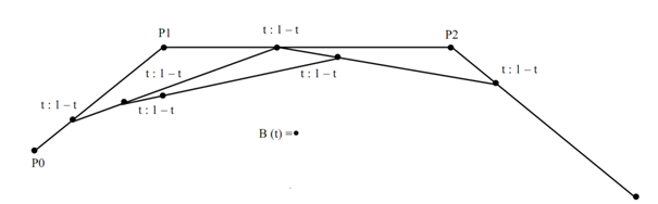
All of them are then divided in the similar ratio t: 1- t, giving rise to another point. Again, all consecutive two are joined along with line segments that are subdivided, till only one point is left. It is the location of our shifting point at time t. The trajectory of such point for times in between 0 and 1 is the Bezier curve.

An easy method for constructing a smooth curve which followed a control polygon p along with m-1 vertices for minute value of m, the Bezier techniques work well. Though, as m grows large as (m>20) Bezier curves exhibit several undesirable properties.

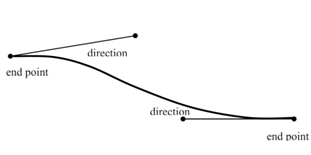
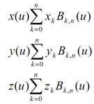
Figure: (a) Beizer curve defined by its endpoint vector    

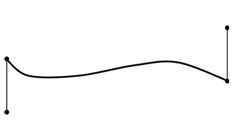
Figure (b): All sorts of curves can be specified with different direction   vectors   at   the   end points

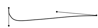
Figure: (c): Reflex curves appear when you set the vectors in different directions

Generally, a Bezier curve section can be suited to any number of control points. The number of control points to be estimated and their relative positions find out the degree of the Bezier polynomial. Since with the interpolation splines, a Bezier curve can be given along with boundary conditions, along with a characterizing matrix or along with blending function. For common Bezier curves, the blending-function identification is the most convenient.

Assume that we are specified n + 1 control-point positions: p_k = (x_k , y_k , z_k ) with k varying from 0 to n. Such coordinate points can be blended to generate the subsequent position vector P(u), that explains the path of an approximating Bezier polynomial function in between p₀ and p_n .

--------------------(1)

The Bezier blending functions B_k,n (u) are the Bernstein polynomials.

 B_{k ,n} (u) = C (n, k )u^k (1 - u)^{n - k}               -------------------(2)

Here the C(n, k) are the binomial coefficients as:

C (n, k ) =  nC_k   n! /k!(n - k )!           -------------------- (3)

Consistently, we can describe Bezier blending functions along with the recursive calculation

 B_{k ,n} (u) = (1 - u)B_{k ,n -1} (u) + uB_{k -1,n -1} (u), n > k ≥ 1      ---------(4)

 Along with BEZ_{k ,k}= u^k , and B_0,k = (1 - u)^k.

Vector equation (1) as in above shows a set of three parametric equations for the particular curve coordinates as:

-------(5)

Since a rule, a Bezier curve is a polynomial of degree one less than some of control points utilized: Three points produce a parabola, four points a cubic curve and so forth. As in the figure 12 below shows the appearance of several Bezier curves for different selections of control points in the xy plane (z = 0). Along with specific control-point placements, conversely, we acquire degenerate Bezier polynomials. For illustration, a Bezier curve produced with three collinear control points is a direct-line segment. Moreover a set of control points which are all at the similar coordinate position generates a Bezier "curve" that is a particular point.

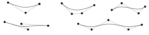
Bezier curves are usually found in drawing and painting packages, and also CAD system, as they are easy to execute and they are reasonably powerful in curve design. Efficient processes for determining coordinate position beside a Bezier curve can be set up by using recursive computations. For illustration, successive binomial coefficients can be computed as demonstrated figure below; through examples of two-dimensional Bezier curves produced three to five control points. Dashed lines link the control-point positions.