Reference no: EM132275444

Heat Transfer Numerical Analysis Problems -

Instructions - Write a report with comments, equations, figures, and algorithms. You are free to organize the plots in an effective manner. Submit all your Matlab scripts in a .zip archive into which you will also include your report.

Introduction - For purposes of heat-sink manufacturing, you are required to perform steady-state and time-variant heat transfer analysis for a rectangular fin design. The heat-sink is made of copper and is assumed to be submerged in an air flow. Specifically, the two-dimensional rectangular fin depicted in Fig. 1 with a uniform (6 x 11) grid of nodes (x_i, y_j) is considered. Point A is located at (0 cm, 0 cm) and point B at (1cm, 2cm). The partial differential equation that represents the heat transfer problem is given by

- ∇ · (k(x, y, T)∇T) = f(x, y) on Ω (1)

where ∇ stands for the gradient differential operator, k(x, y, T) is the spatially varying thermal conductivity of the fin material , and f(x, y), for the heat generated inside the body. Of course, the fin itself generates no heat. However, the edge ∂Ω_B, where the fin is in contact with the heat source:

T = T_∞ + g(x)(T_b - T_∞) on ∂Ω_B (2)

where g(x) describes the temperature profile at the base of the fin. Furthermore, the other sides are in contact with air. As a result, natural convection occurs and convective heat transfer is given by

-k(x, y, T)∇T · n = h(x, y)(T - T_∞) on ∂Ω_L, ∂Ω_R, ∂Ω_T (3)

where h(x, y) denotes the heat transfer coefficient of the surrounding fluid, and n denotes the outward-pointing normal to the boundary. The temperature on edge δΩ_B is kept constant at T_b = 420K with distribution g(x) = 1.05x(1 - x), the ambient air temperature is T_∞ = 370K. Note that x here is given to you in terms of centimeters such that the corner of the base have a temperature of T_∞.

Steady-State Analysis -

We are interested in the temperature distribution throughout the fin by numerically approximating the temperature field T(x, y). Assuming k = k_a and h = h_a are constant. Provide reference and justification for your choice of k_a and h_a:

1. Discretize the problem

(a) Provide the expression of ∇ in Cartesian coordinates.

(b) Using a finite-differences scheme in two dimensions, suggest a second-order accurate approximation of PDE in the domain -∇·(k(x, y, T)∇T) = f(x, y) at point (x_i, y_j) in the domain.

(c) Using a finite-differences scheme in two dimensions, suggest a first-order accurate approximation of the quantity k(x, y, T)∇T·n (boundary condition equation) at point (x_i, y_j) on the boundaries.

(d) For a uniform 3 x 5 grid, write down the 15 equations required to solve the 15 unknowns. Use any notation for temperatures on the grid, explain using a schematic of the surface in Fig. 1.

2. You should have a system of linear equations Ax = b.

(a) Use LU decomposition (code it yourself) to solve this linear system and find the temperature distribution, for grids of size (6 x 11), (16 x 31), (46 x 91), and (61 x 121). One a single plot, show the temperature distribution along the x = 0 axis for all four grids. Note that you may compare your results using backslash \.

(b) In a table, report the total number of unknowns, the CPU time (MATLAB function tic, toc) required to solve the temperature distribution on each grid, and the memory required to store your matrix A (remember that a double requires 8 bytes of storage). Estimate the required time and memory to solve this on a grid of size 181 x 361 using interpolation.

(c) For the (46 x 91) grid, prove that Jacobi converges to the unique solution.

Bonus Question - Use Jacobi, Gauss-Seidel, or SOR to solve for the temperature distribution for grids of size (6 x 11), (16 x 31), (46 x 91), (61 x 121), (181 x 361). Provide the convergence plots of the problem. Compare your results and performance with the Gaussian elimination. Note that to get the any marks, your solver should be coded such that you can solve the (181 x 361) problem.

Transient Analysis -

For transient heat analysis of the fin, it is presumed that heat is dissipated from the object through time. Hence, the heat generated inside the body is now a function of T and time, t:

f(x, y, T, t) = - ρ C_p ∂T/∂t (4)

where ρ is the density of the object and C_p is the object's heat capacity at constant pressure. As well, The temperature profile of the source is time-variant:

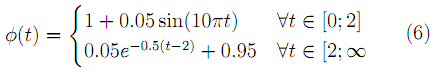
g(x, t) = 1.05x(1 - x)Φ(t) (5)

At last, assume that, initially, the fin is at T_∞ uniformily.

Case 1 - Given

1. Write the numerical scheme for two IVP solvers presented in class applied on a 3 x 5 grid. Plot the temperature for t ∈ [0; 4] at the point (0.3^- cm, 0.4 cm) for both IVPs on the same plot. Discuss the stability and consistency of the chosen IVP solvers.

2. Find the solution at t = 4s using two of the IVP solvers presented in the course. For a grid of 16 x 31 with Δt = 1 x 10^-4. Compare the two methods in terms of convergence to the solution in Δt = 1 x 10^-4 and computation time. Use plots to support your claims.

3. Find the solution as t → ∞. Does the solution converge? Elaborate.

4. Bonus Question - In most engineering applications, it is assumed that k(x, y, T) = k_a(1 - β(T - T_∞)). Without using any numerical computation, how would this affect your choice of solvers for the transient analysis and steady state analysis?

Case 2 -

For Φ(t) = 1, it is possible to construct a scheme such that:

T(t = 0) = T₀

T^· = CT + r (7)

where T represents a vector array of the temperatures used as functions of time. An upper-dot, o^·, denotes differentiation in time. As well, C and r do not depend on time. The system in (7) can be decoupled by performing an eigen-decomposition of the matrix C such that:

C = PDP^-1 (8)

where D is a diagonal matrix containing all eigen-values and P is a matrix containing all corresponding normalized-eigenvectors. Hence, a solution can be represented as:

T(t) = Pe^DtP^-1(T₀ + C^-1r) - C^-1r (9)

Use of MATLAB's backslash function is allowed. For e^Dt please refer to the Wikipedia article Matrix Exponentiation.

1. Show explicitly all the components of equation (7) when applied to a 3 x 5 grid.

2. Using the methods presented in class, develop a scheme to find D and P and find both for a uniform grid of 3 x 5. All eigen-values found in D should be negative. Compare your answers using the eig function in MATLAB.

3. Compare the solution found by your scheme with one of the IVP solvers presented in class. Answer in terms of computation time and accuracy in application to arbitrary grids.

4. Bonus Questions -

1. Should the analytic solution converge to a steady-state solution as t → ∞? Does T (t) for a grid 3 x 5 converge to a steady-state solution? Elaborate.

2. Show that (9) is a solution to (7).

3. Explain why (9) is not representative of the solution for non-constant Φ(t).

Note - Need help with mainly is the "Transient Analysis" part and the bonus questions in each section.

Attachment:- Assignment File.rar