Reference no: EM133366146

Advanced Linear Algebra for Computing

Question 1. Let's have a closer look at Cholesky factorization.

(a) In a "Ponder this" in the notes, a bordered algorithm for computing the LU factorization is discussed. (It is also discussed in Enrichment 5.5.1.) Propose a bordered algorithm for computing the Cholesky factorization of a SPD matrix A inspired by the bordered LU factorization algorithm. Show your derivation that justifies the algorithm. You don't need to use the formalisms in 5.5.1, but you do need to derive the algorithm. You may want to do so by partitioning

Note: you can likely find such an algorithm online or in the literature and that is permit- ted. (Although, you'll learn more if you do the problem using only the notes.) Regardless, you must give your solution with notation that is consistent with the notation we use in our notes.

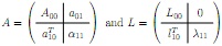
(b) Consider the Cholesky Factorization Theorem discussed in the notes (modified for real- valued matrices):

Theorem Given a SPD matrix A, there exists a lower triangular matrix L such that A = LL^T. If the diagonal elements of L are restricted to be positive, L is unique.

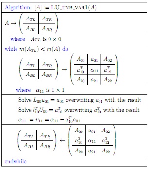
In the notes, we prove this theorem by showing that the right-looking Cholesky factoriza- tion algorithm is well-defined for a matrix A that is SPD. Prove this theorem instead by showing that the bordered Cholesky factorization algorithm is well-defined for a matrix A that is SPD.
Here are some hints:

• Employ a proof by induction on n, the size of the matrix.
• Why is the computation of l^T₁₀ well-defined and uniquely defined?
• What property has to be true about how α₁₁ is updated before λ₁₁ is computed for λ₁₁ to be well-defined?

Note: you can likely find such a proof online or in the literature and that is permitted. (Although, you'll learn more if you do the problem using only the notes.) Regardless, you must given your solution with notation that is consistent with the notation we use in our notes.

Question 2. In this question, we are going to walk you through the backward error analysis of the bordered LU factorization algorithm.

where L₀₀ and U₀₀ have overwritten A₀₀.

The result is, as it is for the Crout variant of LU factorization:

A + ΔA = L^{^}U^{^} with |ΔA| ≤ γ_n|L^{^}||U^{^}|,

where L^{^}U^{^} equals the computed LU factorization of matrix A.

The proof is, of course, by induction. Here is an outline of what you need to do.

(a) Prove the base case: n = 1.
(b) Inductive Step: Assume that for A₀₀ ∈ R^nxn the bordered LU factorization computes (in floating point arithmetic) L^{^}00 and U^{^}00 where
A₀₀ + ΔA₀₀ = L^{^}₀₀ U^{^}₀₀ with |ΔA₀₀| ≤ γ|L^{^}₀₀||U^{^}₀₀|.

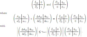
(highlighted in red updated 3/31/2021) Show that when the bordered algorithm is applied to

it computes (in floating point arithmetic)
Notice that in a number of places α₀₀ has been corrected to α₁₁ and u₀₀ to u₁₁

To do so, you will have to figure out which results fr om the notes to use. We don't have results for solving with an upper triangular matrix in the notes, but you can extrapolate what those results would be from the result for solving with a lower triangular matrix.

Hint: Distribute the absolute value operation over the submatrices and multiply out partitioned matrix-matrix multiplications. This will guide you towards the results you need.

Again, you may be able to find such an analysis somewhere, but it is important that you use our notation for this exercise.

Question 3. For this last problem, you will implement various algorithms from Week 8 to solve Ax = b. We start by giving you a number of scripts and functions:

Solve_Poisson_on_unit_square.m: A script that creates the matrix and right-hand side for the problem in Week 7.1.1 (but in matrix and vector form rather than as the mesh.) It then tests the various implementations you will create. You will have to uncomment the obvious lines to do so.

Create_Poisson_problem_A.m: An outline for a function that creates the matrix A for the Poission problem.
A = Create_Poisson_problem_A( N )
(modified 4/2/2021:) where N is the size of the N N mesh (meaning there are N2 interior points).

Place_F_in_b.m: A routine that takes the "load" information (function f in the discus- sion in 7.1.1) and creates a vector b from this. You don't need to write this one. This routine allows us to that the 2D array of values F and extract from this the right-hand side vector b when solving Ax = b.

Place_x_in_U.m: A routine that takes the displacements that are computed, and enters them back into the 2D array U so that we can plot the result.

To keep things simple, matrix A is just stored as a full matrix (with all its zeroes). In practice, that is not what you would want to do.
Now here is what you will be doing:
• Complete the function Create_Poisson_problem_A( N ).
• Write a function that implements the Method of Steepest Descent.
[ x, niters ] = Method_of_Steepest_Descent( A, b )
in Method_of_Steepest_Descent.m. It must closely resemble the algorithm in the notes.
• Write a function that implements the Conjugate Gradient Method (CG).
[ x, niters ] = CG( A, b )
in CG.m. This implements the Conjugate Gradient Method without preconditioning. It must closely resemble the algorithm in the notes.
Next, will implement preconditioned versions of these algorithms:
• Write a function that implement the Method of Steepest Descent.

[ x, niters ] = Method_of_Steepest_Descent_ichol( A, b )

in Method_of_Steepest_Descent_ichol.m. This adds preconditioning with an incom- plete Cholesky factorization.

Rather than having you write your own incomplete Cholesky factorization routine, with all the bells and whistles, you will instead use Matlab's ichol routines. You can read up on it by typing "help ichol" in the command window of Matlab Online.

This routine requires A to be stored in sparse format. Given that we are (foolishly) storing the matrix as a full matrix, you will have to call

L= sparse( ichol( sparse( A ) ) )+.

Here, sparse( A ) converts the full matrix to sparse format and the outer sparse converts it back to the full matrix. (This last one is probably not necessary. Play around with that.)

It must closely resemble the algorithm in the notes.

Write a function that implements the preconditioned Conjugate Gradient Method (PCG) that also uses the incomplete Cholesky factorization.
[ x, niters ] = PCG( A, b )
in PCG.m.

You created an algorithm for this as part of the homework for Week 8.

The sample "driver", in Solve_Poisson_on_unit_square.m, sets up the problem and solves it using Matlab's intrinsic solution operation: x = A \

b. It then also calls the routines that you are to write. Notice that Matlab's \ operator can also be used to solve with a triangular matrix.
You may notice that incomplete Cholesky (which performs Cholesky factorization by skips all steps that would introduce nonzeroes) doesn't really help convergence. There are variations on incomplete Cholesky that create fill-in with some threshold parameter. You may want to play with that:

L = sparse( ichol(sparse(A), struct('type','ict','droptol',1e-2,'michol','off')));

In particular, change the tolerance.

The idea now is to look at the number of iterations needed to convergence. The Method of Steepest Descent and CG each perform one matrix-vector multiplication per iteration. So those are easy to compare. The preconditioned versions also perform the factorization (but only once) and triangular solves (for each iteration). This increases the cost per iteration, but reduces the number of iterations.

Your final part of this assignment is to write a few sentences about what you observed when you ran the experiments. (Regarding iterations to convergence.)

A final hint: In the last unit of Section 8.3 a stopping criteria is discussed. It can be used for all your implementations.