Reference no: EM132357814

Algorithms in Machine Learning Assignment -

Question 1 - A certain type of electronic component has a life time X (in hours) with probability density function given by

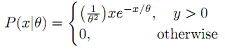
Suppose that three such components, tested independently, had lifetimes of x₁ = 120, x₂ = 130, and x₃ = 128 hours.

(a) Plot the likelihood function P(x|θ) as a function of θ for a single data point x₁. From the plot, comment about the most likely value of θ.

(b) On the same plot in part (a), add the likelihood function for each data point x₂ and x₃. For better visalization, you should use a different colour for each likelihood function.

(c) Write down the likelihood function for N data points P(x₁, x₂, . . . , x_N|θ), then derive the maximum likelihood estimate (MLE) of θ, denoted θ^{^}.

(d) Substitute the values of the given data points x₁, x₂, x₃ into θ^{^} and compare this result with the plot in (b).

Show and justify all working.

Question 2 - To validate the EM algorithm, we'll test it on a synthetic data set where the parameters π_k, μ_k, ∑_k with k = 1, 2 are known. Here we only work with bivariate (or two-dimensional) Gaussians.

Step 1: Generate a sample of size N from a mixture of two bivariate Gaussians. To generate a data point, you pick one of the components with probability π_k, then draw a sample x_i from that component using mvnrnd(). Repeat these steps for each new data point.

Step 2: Implement the EM algorithm given in the lectures for this synthetic data set. Label your script file my_em.m. Plot your resulting mixture of Gaussians. Are your results closed to the true parameter values?

Step 3: Repeat the Steps 1 and 2 for B = 100 times but keep the same parameter values π_k, μ_k, ∑_k. Calculate the means of the estimates for each parameter π_k, μ_k, ∑_k and present them in a table. Comment about your results.

Question 3 - Revisit the Question 3 in Assignment 1, you toss a bent coin N times, obtaining a sequence of heads and tails. The coin has an unknown bias f of coming up heads.

We assume the prior for f is a beta distribution (Mackay section 23.5 or Bishop 2.1.1), Beta(α, β). The probability density function of the beta distribution is given by the following:

P(f|α, β) = (f^α-1(1-f)^β-1)/B(α, β)

Where the term in the denominator, B(α, β) is present to act as a normalising constant so that the area under the PDF actually sums to 1.

(a) Show that the posterior distribution of f, P(f|n_H), is also a beta distribution. Show and justify all working.

(b) We carried N = 50 tosses and observed n_H = 12 heads. Plot the prior Beta(12, 12) and the resulting posterior distribution about P(f|n_H) on the same figure.

(c) Implement a Markov chain using the Metropolis method given in the lectures to simulate from the posterior distribution. Label your script file my_metropolis.m. Then compare the results from a closed-form solution in (b) and one calculated by numerical approximation. Plot the analytic and MCMC-sampled posterior distributions about f, overlaid with the prior belief.

Note - Use MATLAB to solve the questions for plotting.