Goods Market and the IS Curve

The IS curve shows the combinations of interest rates and levels of output such that planned spending equals income. In order to derive the IS curve, first we will have to drop the simplifying assumption made earlier of investment being autonomous. We will have to consider explicitly the determinants and the functional form of investment.

Investment is spending on additions to a firm's capital, such as machines, or buildings. Typically, firms borrow to purchase investment goods. The higher the interest rate for such borrowing, the less they will be willing to borrow and invest. Conversely, firms will want to borrow and invest more when interest rates are lower. Let us assume that the investment spending function is of the form

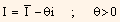
Where i is the rate of interest and θ  measures the responsiveness of investment to changes in interest rate.     denotes autonomous investment spending, that is, independent of both income and interest rate.

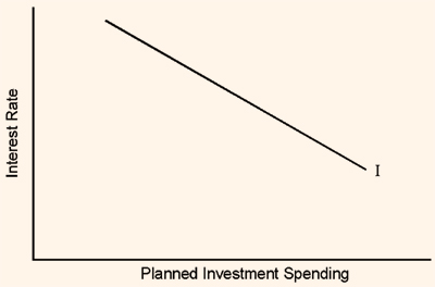
From the equation it can be seen that the lower the interest rate, the higher is the planned investment and vice versa. Figure 5.1 shows the investment schedule. The schedule shows the amount of planned investment expenditure for various levels of interest rates.

Figure 

Derivation of the IS Curve

First of all, we will have to modify the aggregate demand function of the earlier chapter to reflect the new planned investment spending schedule.

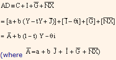
For equilibrium in the goods market

Y       = AD

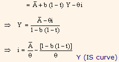
From the above equation we can see that when the interest rate increases, the equilibrium output decreases and vice versa. The set of combinations of income (Y) and interest rates (i) which represent the equilibrium in the goods market is called the IS curve.

Figure 5.2 (a)

We can draw the IS curve using a different approach.

Figure 5.2 (b)

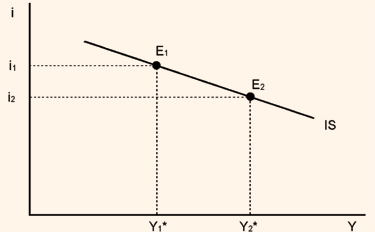
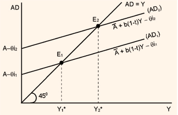
In the upper part of figure 5.2, we have shown two aggregate demand schedules corresponding to two different rates of interest. When the interest rate is i1, the aggregate demand schedule AD₁ cuts the 45^o line at E₁ and the corresponding equilibrium income in Y₁*. This combination of interest rate i₁ and income Y₁*gives rise to an equilibrium in the goods market and is shown in the lower part of figure 5.2, by the point E₁. When the interest rate falls from i₁ to i₂, the investment demand increases as a result of lower interest rate. This pushes up the aggregate demand curve upwards and is shown by AD₂. AD₂ cuts the 45^o line at E₂. The output Y₂* corresponding to the point E₂ is an equilibrium output when the interest rate is i₂. i₂ and  Y₂*  are shown in the lower part of the figure by point E₂. In a similar manner, other combinations of interest rates and income which produce goods market equilibrium can be got. Joining all these points gives us the IS curve.

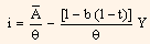
Now, let us derive some important properties of the IS curve. The equation of the IS curve is

since the multiplier

we can rewrite the equation of the IS curve as

From the above equation it can be seen that the steepness of the IS Curve depends on the multiplier ( α ) and investment sensitiveness to changes in interest rates (  θ  ). We see that if  θ   is large, then the IS Curve would be flat because    would be small. It can also be inferred that larger the multiplier, the flatter would be the IS curve. Since the slope of the IS Curve is dependent on the multiplier and the multiplier in turn is dependent on fiscal policy - more specifically, the tax rate 't' - we see that fiscal policy can affect the slope of the multiplier. An increase in the tax rate would reduce the multiplier, which in turn increases the steepness of the IS Curve. Thus, the steepness of the IS Curve and the tax rate go in the same direction.

Now, let us see the effect of an increase in autonomous expenditure of the IS Curve. An increase in autonomous expenditure would increase the term     in the equation for IS curve and thus an increase of    . A rise in     would mean an outward shift, that is to the right, of the IS Curve. Thus, for example, an increase in autonomous government expenditure would result in an outward shift of the IS Curve.

We can sharpen our understanding of the meaning of the IS Curve by considering points off it - that is points not on the IS Curve.

Figure 5.3

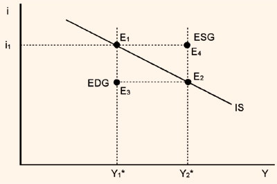
Now, in figure 5.3 points E₃ and E₄ are disequilibrium points because they do not lie on the IS Curve. What are the properties of points E₃ and E₄? Let us first consider point E₃. Point E₃ has the same level of income as point E₁, but the interest rate is lower. Therefore, the demand for investment is higher at E₃ than at E₁. Consequently, the aggregate demand is higher at E₃than at E₁. Since at E₁, an equilibrium point, quantity demanded is equal to quantity produced, at E₃ quantity demanded will have to be greater than quantity produced. Thus at E₃, have excess demand for goods and services over what is supplied. What applies to E₃ applies to all points below the IS Curve as well. A similar reasoning can be used to show that at all points above the IS Curve, we have excess supply of goods, that is, aggregate demand is less than output.