Cases for Digital Differential Analyzer Algorithm

1)  If in case 1, we plot the line another way round that is, moving in y direction via 1 unit every time and after that hunting for x direction pixel that best suits the line. In this condition, all times we look for the x pixel; this will offer more than one option of pixel and hence enhances the defect of the stair case consequence in line generation. Moreover, from the figure of DDA line generation, we notice that in another way round strategy for plotting line 1, the vertical span is fairly less in comparison to the horizontal span. Hence, a lesser number of pixels are to be completed ON, and will be accessible if we increase Y in unit step and may be X. Although more pixels will be accessible if we raise X in unit steps and approximate Y such option will also decrease staircase consequence distortion in line generation, so more motion is to be made beside x-axis.

2) identify a line to be generated from (X₀, Y₀) to (X₁, Y₁). If

 (X₁ - X ₀ > Y₁ - Y₀) and X₁ - X₀ > 0 then slope (m) of line is < 1 thus case 1  for line generation is applicable or else case 2, that is If ( X₁ - X₀  < Y₁ - Y₀ ) and X₁ - X₀ > 0 then slope m > 1 and case 2 of line generation is appropriate.

Important: Assume as X₁>X₀   is true else swap (X₀, Y₀) and (X₁, Y₁)

3)   When 0 < m < 1: increment X in unit steps and approximate Y

Unit increment must be iterative ⇒ x_i = (x_i - 1) + 1 hence (x_i, y_i) resolves to (x_i, mx_i + c) or (x_i, mx_i) . This is to be noticed that whereas calculating y_i, if y_i became to be a floating number then we round its value to choose the approximating pixel. Such rounding off feature gives to the staircase consequence.

While infinity > m > 1 increment Y in unit steps and estimated X, simplify (x_i, y_i) as per.

Case 1: slope (m) of line is < 1 or 0 < m < 1

Identify a line to be made from (X₀, Y₀) to (X₁, Y₁), suppose that X₁>X₀ is true else swap (X₀, Y₀) and (X₁, Y₁). Now, if (X₁ - X₀ > Y₁ - Y₀) it implies slope (m) of line is < 1 thus, case 1 for line generation is valid. Therefore, we require increment X in unit steps and approximating Y. Consequently from X₀ to X₁ , x_i is increased in unit steps in the horizontal direction, there for these unit steps the appropriate value of Y can be estimated through the common equation of line y = mx + c.

Likewise, for case 2, let we discuss for sum up our discussion on Digital Differential Analyzer algorithm for both cases. We will check all cases separately.

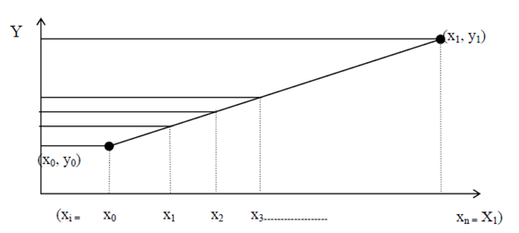
Figure: Slope (m) of line is < 1 (i.e., line 1)

 Sum -up

For illustration, in a specified line the end points are (X₀, Y₀) and (X₁, Y₁). Utilizing these end points we determine the slope (m = Y₁ - Y₀/ X₁ - X₀) and confirm that the value of m lies among 0 and 1 or is > 1. If 0 < m < 1 so then case 1 applies, else, case 2 applies.

For case 1: increase x in one Unit all times.

For case 2: increase y via one Unit all times and approximate respective values of y and x.

We suppose equation of line is y = mx+c

At x = x_i; we have y_i = mx_i+c

Similarly at x = x_i + 1; we have y_i + 1 = mx_i + 1 +c

Case 1: Slope (m) of line is 0 < m1 (that is line 1)

Because x is to be increase via 1 unit all times

⇒ x_i + 1 = x_i + 1                            -----------Eq. (1)

Consequently by utilizing equation of line y = mx+c we have y_i + 1 = m (x_i + 1) +c

= mx_i +c + m

= y_i + m                        ------------ Eq.(2)

Eq(1) and Eq(2) means that to approximate line for case 1 we should move along x direction via 1 unit to comprise subsequent value of x and we should add slope m to firstly y value to acquire subsequent value of y.

Now, by using the starting point (x₀, y₀) in the above eq(1) and Eq(2) we go for x_i and y_i (i = 1, 2, ......n) and place colour to the pixel to be lightened.

This is assumed as X₀ < X₁ ∴the algorithm goes like:

It is assumed that X0 < X1 ∴the algorithm goes like:

x ← X0

y ← Y0

m ← (Y1 - Y0)/ (X1 - X0)

while (x < = X1) do

{           put-pixel (x, round (y), color)

(new x-value) x ←  (old x-value) x + 1 (new y-axis) y ← (old y-value) y + m

}

Sample execution of algorithm case 1:

At (x₀, y₀): put-pixel (x₀, y₀, colour)

x₁ = x₀ + 1;        y₁ = y₀ + m

Likewise, x₂ = x₁ + 1; y₂ = y₁ + m

At (x₂, y₂): put pixel (x₂, y₂, colour) etc.

Case 2: slope (m) of line is > 1 (that is line 2): Similar as case 1 although, this time, the y component is raised by one unit all times and suitable x component is to be selected. To do the task of suitable selection of x component we utilize the equation of Line: y = mx+c.

Unit increment must be iterative ⇒ y_i+1 = y_i + 1 ; for this y_i+1 we determine consequent xi+1 by utilizing equation of line y = mx + c  and thus get next points (x_i+1, y_i+1).

⇒ y_i + 1 - y_i = m (x_i + 1 - x_i)          ----------- (3)

As y is to be raise by unit steps

∴y_i + 1 - y_i = 1                           ----------- (4)

By using Eq(4) in (3) we get

⇒ l = m (x_i + 1 - x_i)                      ----------- (5)

Rearranging here Eq.(5) we obtain:

⇒ 1/m = (xi + 1 - xi)

x_i+1 = x_i +1/m

Consequently, procedure as a whole for Case 2 is totaled up as Algorithm case 2: suppose Y₀ < Y₁ the algorithm goes like

Algorithm for case 2:

x ← X0;

y  ← Y0;

m ← (Y1 - Y0)/ (X1 - X0);

m1 ← 1/m;

while (y < Y1) do

{

put-pixel (round (x), y, colour)

y ← y + 1;

x ← x + m1;

X     

}

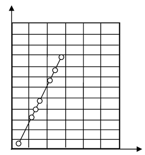
                                                                        Figure: Slope (m) of line is > 1