Reference no: EM132363676

Assignment

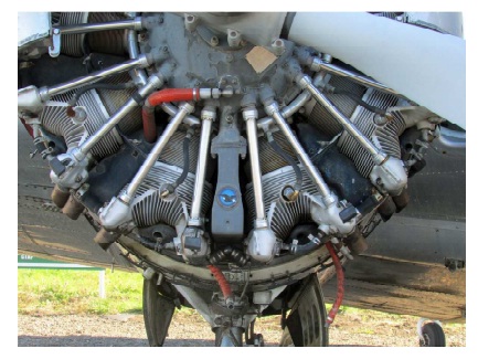
In this assignment you will investigate how heat is transferred between air and a cooling fin on an aircraft engine radiator. The scenario considered is shown in the figure below.

In this assignment you will solve this problem using the finite element method using Matlab.

The assignment is arranged into two parts:

In Part A you will determine the steady state temperature on a single fin. You will approximate the fin as a one dimensional plate. You will obtain solutions using the Galerkin Finite Element method using quadratic trial functions and writing a Matlab script to solve the equations. Your goal is to determine the temperature at the end of the fin and demonstrate your code is accurate by comparison with an exact solution.

In Part B you will examine the two dimensional heat transfer within the air itself. You will use the Galerkin Finite Element method to obtain discrete equations for this problem using linear triangular elements and then write a Matlab script to solve this problem based on your code for Part A. You will use the mesh generator in Matlab.

You will present your results in a short report. In this report you must briefly explain your method, the discrete equations solved, how boundary conditions were applied, explain what simulations were performed, what settings were used. In particular you must show how you
determined your solution is accurate by giving tables of results and showing convergence of results with element size. Details for each part are given in the following pages.

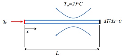
PART A) In this section you will demonstrate that you can write Finite Element Code to solve a much simplified approximation of this problem for which an exact solution exists. You are to approximate the heat transfer along the fin as one dimensional and use the simplified geometry below:

The one dimensional steady heat equation for this problem is

k(d²T/dx²)-(2W/A_c) h (T(x)- T_∞) = 0

where W is the width (into the page dimension) of the fin, B is the thickness of the fin, A_c = W B is the fin cross-sectional area (m² ). The equation can be simplified using θ(x) = T(x) − T_∞,

d²θ/dx²-α²θ=0

with α² = 2h/κB = 200 (m⁻²) for this approximation. In this approximation make the further approximation that boundary conditions are q_c(x = 0) = 110, 000 W/m² , the fin alloy has a conductivity of κ = 200 (W/mK) and assume dT(x=L) dx = 0 and that L = 0.04 m.

Your task is to solve this problem use the finite element Galerkin method with quadratic trial functions and compare your solution with an exact solution.

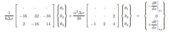
1. Derive the element stiffness matrix and load vector for this problem. Present your derivation of each term and present the equations in matrix form i.e. [k][θ] = [f]. The result will look similar to the result below. Derive only the terms missing from the result below (fill in the dots).

2. Show how to assemble the global element equations for two elements and apply boundary conditions. (include in the report appendix)

3. Write a Matlab script to solve the set of equations for an arbitrary number of elements.

An incomplete example code will be provided. Your code should include the assembly process, apply the correct boundary conditions and solve the global system of equations.

The code should be extensively commented.

4. Compare your FEM code result by plotting T(x) for 2 elements with the exact solution.

[HINT: A general solution of governing equation is: θ = C₁e^αx + C₂e^−αx ].

5. Run your FEM code with a range of element sizes: Ne = 1, 2, 4, 8, 16 elements. Calculate the error in your simulations at the location x = L. Plot the error with element size. The error is e(x) = θ(x) − ˜θ(x) where ˜θ(x) is the numerical result.

6. Using the above results write a short ∼ 3 page report. Your report should :

(a) present your numerical method including the final element stiffness matrix and load vector. Show how you implement the boundary conditions in the final assembled equations. Your derivations of the element equations can be hand written (neatly) and included as an appendix to your report.

(b) present your solution T(x) and the result at T(x = L).

(c) demonstrate the accuracy of your solution using plots and tables.

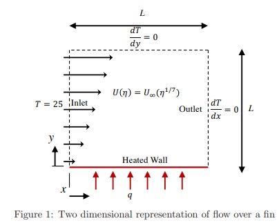
PART B) In this section you will simulate the transport of heat in the air flow along the cooling fin. The flow of air over the heated fin surface is depicted in figure 1. The fluid enters the domain with a constant velocity profile U(η) = U_∞(η ^1/7) with U_∞ = 3 m/s where η = y/δ and δ = L = 0.05 m.

The air at the inlet as a constant inlet temperature of T = 25 ^?C. The lower wall indicated by red line is the heated fin surface. This fin heats the air with a constant uniform heat flux of 500 W/m².

The steady transport of heat in a flowing fluid is described by the steady advection diffusion equation which in two dimensions can be written as follows,

U(∂T/∂x) + V(∂T/∂y) = α (∂²T/∂x²) + (∂²T/∂y²)

where α = 1.0×10⁻³ m²/s is the thermal diffusivity and U and V are the x and y components of velocity. The thermal conductivity of air is κ_a = 0.026 W/mK. For the present problem V = 0 and the velocity in y is given by,

U(η)=U_∞(η^1/7)

For the present flow problem the boundary conditions for T are,

y-boundaries:

Heated Wall : (∂T/∂y)|_y=0  = -(qN/κ_a),   Top Boundary : (∂T/∂y)|_y=L  = 0,

x-boundaries:

Inlet : T|_x=0 = 25,  Outlet : (∂T/∂x)|_x=L = 0,

Your task is to solve this problem use the finite element Galerkin method with two dimensional linear triangular elements and determine the temperature distribution along the fin. You should also approximate the velocity field U using linear triangular elements i.e

U(x, y) = N₁(x, y)U₁ + N₂(x, y)U₂ + N₃(x, y)U₃.

Use the supplied velocity profile to determine the nodal values of velocity for each element. This approach will make the integration easier and will not significantly reduce the accuracy of our solution.

1. Derive the element stiffness matrix and load vector for this problem. Present your derivation of each term and present the equations in matrix form i.e. [k][θ] = [f]. Derive the discrete form of the boundary conditions for each type of boundary condition in this problem.

2. Draw the fin using the Matlab pdetool package. Mesh the object you have drawn and export the mesh files : p, e, t arrays. Save the mesh to file:

>> save(‘lastnameSIDMesh.mat’,‘e’,‘p’,‘t’);

3. Write a Matlab script to solve the set of equations for an arbitrary number of elements. Your code should include: the import of the mesh (you don’t have to automate the mesh generation step), the assembly process, apply the correct boundary conditions and solve the global system of equations. To import the mesh you might like to use:

>> load(‘lastnameSIDMesh.mat’);

4. Run the code and produce a contour plot of the temperature on the fin. You might like to use the Matlab trisurf function.

5. Refine your mesh and run your code again. Repeat this until you are satisfied with your solution.

6. Present your results with line plots and contour plots. Plot the temperature along the edge of the fin.

7. Using the above results write a short ∼ 3 page report presenting your solution T(x, y)  and in particular the temperature on the fin. You should briefly present your numerical method including the discrete equations and boundary conditions. Your derivations of the element equations can be hand written (neatly) and included as an appendix to your report.

LEARNING/ASSESSMENT OBJECTIVES

1. Understand how to derive discrete equations and boundary conditions for the 1D/2D Finite element method.

2. Understand how to write a Matlab script to solve a Finite element method problem.

3. Understand what mesh generator output looks like and how to use this to solve a FEM problem.

4. Understand numerical accuracy and benchmarking/code verification against analytical and other numerical solutions.

5. Understand how to present a numerical solution and discuss accuracy.