Reference no: EM132590862 , Length: 3 pages
ECH3119 Numerical Methods And Optimization Process
Question 1:
Write a computer program to compute the profile of the concentration in a given tank as shown in Figure 1.
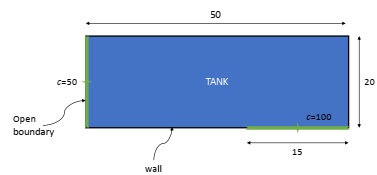
Figure 1: diagram of the tank
The system can be described based on the following partial differential equations:
D (∂2c/∂x2 + ∂2c/∂y2) - kc = 0
and the boundary conditions are as shown. Use suitable value for Δx and Δy to get a accurate results and use value of 0.63 for D and 0.09 for k. Plot the results using a three-dimensional plotting routine where the horizontal plan contains the x and y axes and the z axis is the dependent variable c.
Question 2:
A layer of oil-water that is initially not flowing is placed in between two plates 10 cm apart as shown in Figure 2. At t = 0, the top plate is moved at a constant velocity of 7.5 cm/s. The partial differential equations governing the motions of the fluids are
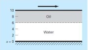
Figure 2: Two plates with the oil-water layer
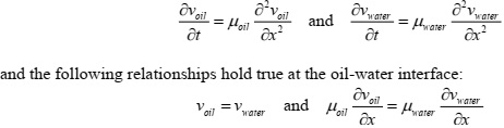
Write a computer program to compute the velocity profile of the two fluid layers at t = 0.5, 1 and 1.5 s at distances x = 2, 4, 6 and 8 cm from the bottom plate. Note that μwater and μoil are 1.7 and 4.3 cp, respectively. Plot the velocity v for oil and water versus length x for various values of time t.
Question 3:
The Poisson equation as shown in the equation below governing the displacement of a uniform membrane subject to a tension and a uniform pressure:
∂2z/∂x2 + ∂2z/∂y2 = -P/T
Write a computer program to solve for the displacement of a 2-cm square membrane that has P/T = 0.6/cm and is fastened so that it has zero displacement along its four boundaries. Employ suitable value for Δx and Δy to obtain accurate results. Display your results as a contour plot. Simulate for P/T = 0.5/cm and P/T = 1.0/cm
Question 4:
Determine the temperature profile along an insulated composite rod that consist of two parts. The nondimensional transient heat conduction equations for the composite rod are given in the equations below:
∂2u/∂x2 = ∂u/∂t 0 ≤ x ≤ 1/3
r∂2u/∂x2 = ∂u/∂t 1/3 ≤ x ≤ 1
where u = temperature, x = axial coordinate, t = time, and r = ka/kb. ka and kb are the thermal conductivity for part a and b. The boundary and initial conditions are
|
Boundary Conditions
|
u (0, t ) = 1.5
|
u (1, t ) = 1.5
|
|
|
(∂u/∂x)a = (∂u/∂x)b x = 1/3
|
|
Initial Conditions
|
u ( x, 0) = 0 0 ≤ x ≤ 1
|
Use second-order accurate finite-difference analogues for the derivatives with a Crank-Nicholson formulation to integrate in time. Write a MATLAB code for the solution, and select values of Δx and Δt for accurate results. Plot the temperature u versus length x for various values of time t. Generate a separate curve for the following values of parameter r = 1, 0.1 0.01, 0.001, and 0.0001.
Question 5:
Apply Alternate Direction Implicit (ADI) method to solve for the temperature profile in an insulated plate. The governing equation is
∂2u/∂x2 + ∂2u/∂y2 = ∂u/∂t
where u = temperature, x and y are spatial coordinates and t = time. The boundary and initial conditions are
|
Boundary Conditions
|
u ( x, 0, t ) = 0
|
u ( x,1, t ) = 1
|
|
|
u (0, y, t ) = 0
|
u (1, 0, t ) = 1
|
|
Initial Conditions
|
u ( x, y, 0) = 0 0 ≤ x < 1 0 ≤ y < 1
|
Write a MATLAB code to implement the solution. Plot the results using a three-dimensional plotting routine where the horizontal plan contains the x and y axes and the z axis is the dependent variable u. Construct several plots at various times, including the following: a) the initial conditions; b) one intermediate time, approximately halfway to steady state; and c) the steady-state condition.