Reference no: EM132292967

Question 1. Let θ ∈ [0, 1] be a constant and denote t_n+θ = (1 - θ)t_n + θt_n+1. Consider the generalised midpoint method

y_n+1 = y_n + hf (t_n+θ, (1 - θ)y_n + θy_n+1),

and the theta-method

y_n+1 = y_n + h[(1 - θ)f (t_n, y_n) + θf (t_n+1, y_n+1)],

for the solution of

(1) y' = f (t, y), t ∈ (a, b]
     y(a) = y0.

(a) Suppose that y ∈ C³[a, b]. Find the truncation error for each method and show that both methods are of order two iff θ = 1/2.

(b) Show that the methods are absolutely stable for any mesh-size h when θ ∈ [1/2, 1]. Determine the intervals of absolute stability of the methods when 0 ≤ θ < 1/2 .

(c) Consider the trapezoidal method, that is the θ-method for θ = 1/2. Consider the model problem

y' = λy, t > 0
y(0) = 1

with a real constant λ < 0. Show that the solution of the trapezoidal method is

y_n = ((1 + 1/2λh)/(1 - 1/2λh))ⁿ,n ∈ N.

Rewrite the solution formula as

y_n = exp((log(1 + 1/2λh) - log(1 - 1/2λh)/h)t_n

and use Taylor polynomial expansions of log(1 ± u) about the point u = 0 to show that

(2) y(t_n) - y_n = -1/12h²λ³t_ne^λt_n + O(h⁴).

So for h small, the error is almost proportional to h².

Question 2. Consider the initial value problem

(3) y'(t) = -y(t) + 2 cos(t), t ∈ (0, 1]
     y(0) = 1.

(a) Apply an appropriate method for solving first-order ordinary differential equations to show that the exact solution of the IVP (3) is y(t) = sin(t) + cos(t)). Write a Matlab function to implement it.

(b) Apply the forward Euler method to solve the above IVP numerically. Use the feuler.m Matlab function discussed in the IT sessions:

function [tnodes,y] = feuler(f, t_interval, N, y0)

y= y0;
yold=y0(:); %initial conditions

t0 = t_interval(1);
tN = t_interval(2);

h=(tN- t0)/N; %mesh-size

tnodes = linspace(t0, tN, N+1); %the nodes of the partition

for tn = tnodes(1:end-1)
ynew = yold+h*feval(f,tn,yold);

y =[y; ynew.'];
yold = ynew;

end

Plot the exact solution and the numerical approximations. Verify that the forward Euler method converges with order one by finding the Experimental Order of Convergence (EOC) (Use the code provided in the IT Sessions). Present your results in a table (see, for example, Table 1) and discuss them.

The Forward Euler Method

h                   Error: max1≤n≤N |y(t_n) - y_n|   EOC
0.5
0.25
0.125
0.0625
0.03125

Table 1: An example

(c) (i) Apply the implicit Euler method to solve the above initial value problem numerically. Use the imp euler.m Matlab function discussed in the IT sessions:
function [tnodes,y] = imp_euler(f, t_interval, N, y0) y= y0;
yold=y0(:); %initial conditions

t0 = t_interval(1);
tN = t_interval(2);

h=(tN- t0)/N; %mesh-size
tnodes = linspace(t0, tN, N+1); %the nodes of the partition

%options = optimset('Display','off');

for tnew = tnodes(2:end)
FixedPointFunction = @(x)odefun(x,tnew,f,yold,h);

%ynew = fsolve(FixedPointFunction,yold, options);

ynew = fsolve(FixedPointFunction,yold);

y =[y; ynew.'];

yold = ynew;
end

function rhs = odefun(x,tnew, f,yold,h)

rhs(:)= x(:)-h.*f(tnew,x)-yold(:);

Plot the exact solution and the numerical approximations. Verify that the implicit Euler method converges with order one by finding the Experimental Order of Convergence (EOC). Present your results in a table (see, for example, Table 1) and discuss them.

(ii) Use the Matlab function imp euler.m as the main ingredient for the implementation of the trapezoidal method

y_n+1 = y_n + h/2(f (t_n, y_n) + f (t_n+1, y_n+1) ,

in a Matlab function my trapezodial.m. Use the Matlab my trapezoidal.m to compute numer- ical approximations to the solution of (3). Verify that the trapezoidal method converges with

order two. Present your results in a table and discuss them. [10]

Question 3. (a) The Butcher table of the improved Euler is

(i) Show that the interval of absolute stability for the improved Euler method is -2 < hλ < 0.

(ii) Show that this method is consistent.

(iii) Use Taylor expansions to show that this method converges with order two.

(iv) Write a Matlab function my improved euler.m to implement the improved Euler method. In- vestigate numerically your theoretical results and report your findings.

(b) The Butcher table of the modified Euler is

(i) Determine the interval of absolute stability for the modified Euler.

(ii) Write a Matlab function my modified euler.m to implement the modified Euler method. Inves- tigate experimentally the stability and discuss your findings.

(iii) Verify experimentally that the modified Euler method converges with order two. Present your results in a table.

(c) The Butcher table of Heun's method is

(i) Write a Matlab function my heun.m to implement the third order Heun's method and verify experimentally that the method has order of convergence equal to three with respect to h. Present the results in a table.

(d) The Butcher table of the Kutta's third order method is

Write a Matlab function my k3.m to implement the Kutta's third order method and verify experi- mentally that the method has order of convergence equal to three with respect to h.

(e) The Butcher table of the classic RK fourth-order method (RK4) is

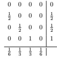
Write a Matlab function my rk4.m to implement the RK4 method and verify experimentally that the method has order of convergence equal to four with respect to h. Present the results in a table.

(f) Consider the solution of the IVP

(4) y' = (1/(1 + t²)) - 2y², t ∈ (0, 1]

    y(0) = 0.

(i) Show that the analytical solution of the above IVP is y(t) = t/1+t².

(ii) Apply all the aforementioned numerical methods to compute approximations to the solution of the IVP (4). Verify the values (to six decimal places) given in Table 1 for t1 with h = 0.1 and the methods shown. Comment on the numerical results. Plot all the numerical approximations

Table 2:

and the exact solution in the same graph.

Question 4. (Implicit - explicit Euler method.) We write an initial value problem in the form
        y' = f (t, y) + g(t, y), a ≤ t ≤ b,

               y(a) = y⁰,
i.e., we decompose the right-hand side of the ODE into two parts. With the usual notation, consider the following method for problem (5)

y_n+1 = y_n + hf (t_n+1, y_n+1) + hg(t_n, y_n), n = 0, . . . , N - 1,

with y0 := y⁰. Obviously, method (6) is a combination of the implicit and the explicit Euler methods, and it reduces to them, when g = 0 and f = 0, respectively. Prove that the order of accuracy of the new method is one, equal to the order of the methods we combined to construct it. Assume now that f satisfies the one-sided Lipschitz condition

∀t ∈ [a, b] ∀z, w ∈ R (f (t, z) - f (t, w))(z - w) ≤ 0,

and g satisfies the global Lipschitz condition with constant L, that is

∃L ≥ 0 ∀t ∈ [a, b] ∀z, w ∈ R |g(t, z) - g(t, w)| ≤ L|z - w|.

Prove d convergence (error estimate) of the method.

[Hint: Use the ODE to check that
y(t_n+1)-y(t_n) - hf (t_n+1, y(t_n+1)) - hg(t_n, y(t_n))
=y(t_n+1) - y(t_n) - hy'(t_n+1) - h[G(t_n+1) - G(t_n)]

with G(t) := g(t, y(t)).]

[Comment: In some cases, when the functions f and g exhibit different behaviour, method (6) com- bines the advantages of both methods, from which it was constructed, without inheriting their draw- backs. For instance, if we use only the explicit Euler method, the constant in the error estimate nec- essarily depends also on f. On the other hand, if f is, e.g., linear, the computation of yn+1 in (6) is very easy, while if we use only the implicit Euler method and g is nonlinear, then to advance in time we
need to solve a nonlinear equation at every time level.]

Question 5. Consider the initial value problem

 y' = λy(t) + g'(t)) - λg(t), t ≥ 0,

 y(0) = y0,

where λ ∈ C, Re λ << 0.

(a) Show that f (t, y) := λy + g'(t)) - λg(t) satisfies a global Lipschitz condition with respect to the y-variable with Lipschitz constant L = |λ|.

(b) Show that the exact solution of (7) is given by

y(t) = g(t) + e^λt(y0 - g(0)), t ≥ 0.

Note that the exact solution has two components, g(t) and e^λt(y₀ - g(0)). If g(t) does not change rapidly over time and λ << 0, i..e. the Lipschitz constant is large, the second component of the solution is negligible with respect the first one for t large enough. On the other hand, the second component, which generally is small and does not influence the behaviour of the solution y(t), changes rapidly for t in the vicinity of 0. Differential equations of the above form with λ negative but large in magnitude are examples of stiff differential equations. When we apply a numerical method to approximate the solution of stiff differential equations, the truncation error may be satisfactory small with not too small a value of h, but the large size of λ , depending on the stability properties of the numerical method, may force h to be much smaller in order that h¯ := λh is in the stability region.

(c) Consider the stiff problem

(8) y' = λy(t) + (1 - λ) cos(t) + (1 - λ) sin(t), t ≥ 0,

y(0) = 1,

whose exact solution is y(t) = sin(t) + cos(t). Notice that the exact solution does not depend on the parameter λ.

(i) Apply the forward Euler method to approximate the solution of the above IVP. Consider the problem (8) with λ = -1, -10, -50. Find an upper bound on the mesh-size h that guarantees stability for the forward Euler method applied to each of the three problems. Use the feuler.m Matlab function discussed in the IT sessions (see the code below) to investigate numerically your theoretical results. Consider the cases h = 0.5, 0.1, 0.01. Report the results for t = 1, 2, 3, 4, 5, as in Table 2. Report your findings.

(ii) Apply the backward Euler method to approximate the solution of the above IVP. Consider the problem (8) with λ = -1, -10, -50. Use the beuler.m Matlab function discussed in the IT sessions (see the code below) and consider again the cases h = 0.5, 0.1, 0.01. Report the results for t = 2, 4, 6, 8, 10 as in Table 2. Report your findings.

(iii) Apply the trapezoidal method to approximate the solution of (8). Consider again the cases h = 0.5, 0.1, 0.01 and report the results for t = 2, 4, 6, 8, 10 as in Table 2.

 y' = f (t, y), t ∈ (0, T ]
 y(0) = y0.

Use the Matlab my trapezoidal.m to find numerical approximations to the solution of (3). Verify that the trapezoidal method converges with order two. Present your results in a table. Report your findings.

Question 6. (a) Let M ∈ R^m×m be a negative semidefinite matrix, x^T M x ≤ 0 for x ∈ R^m. Consider the initial value problem

y'(t) = M y(t), t ≥ 0,

y(0) = y0.

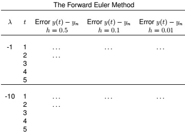
Table 3: An example

(i) Show that the Euclidean norm "y(·)" is a decreasing function.

(ii) With the usual notation, consider the approximations y_n, n ≥ 0, produced by the implicit Euler method with a fixed time-step h > 0. Show that the implicit Euler method mimics the continuous problem, in the sense that "yn+1" ≤ "yn", n ∈ N.

(iii) Consider the approximations yn, n ≥ 0, produced by the trapezoidal method with a fixed time-step h > 0. Show that the method mimics the continuous problem, in the sense that ||yn+1|| ≤ ||yn||, n ∈ N.

(b) Consider the initial value problem

x'(t) = -2x(t) + y(t), t ≥ 0,
y'(t) = 2x(t) - 2y(t), t ≥ 0,
x(0) = x⁰, y(0) = y⁰.

Show that the matrix 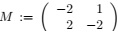is negative definite to conclude that x²(t) + y²(t) is decreasing. Verify numerically the theoretical results derived in (a).

Question 7. Determine the coefficients α₁, α₂, β₂, β₁, β₀ of the general two-step method

y_n+2 + α₁y_n+1 + α₀y_n = h(β₂f_n+2 + β₁f_n+1 + β₀f_n)

such that its order p be at least two, at least three, and at least four, respectively. Does there exist a method with p = 4? Does there exist a method with p = 5? Are the resulting methods stable?

Question 8. Determine the values of the parameter α for which the three-step method

y_n+3 - (α + 1)²yn+2 + α (α² + 2α + 2)yn+1 - α²(α + 1)yn = hf (tn+3, yn+3) is stable.