Reference no: EM133523395

Question 1 The ball and beam system (see Figure 1) has been used frequently in testing different control algorithms.

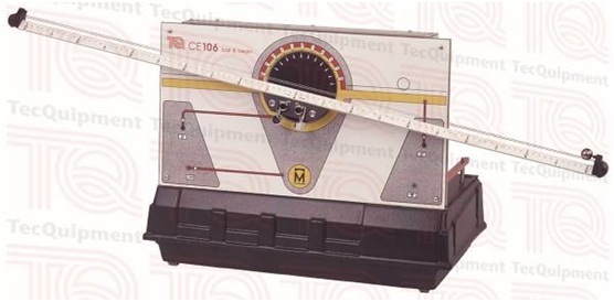
Figure 1

Figures 2 and 3 illustrate the model of the system.

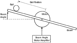
Figure 2

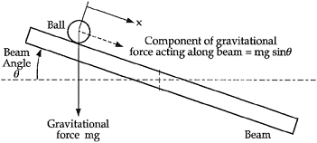
Figure 3

The model of the ball and beam system can be simplified as

mx¨ = mg sinθ,

Where x is the position of the ball, and θ is the beam angle. The beam angle can be assumed to be proportional to the control input u (the motor angle control voltage), and the g is the acceleration caused by gravity. That is

θ = u/g

The position of the ball can be measured by a special sensor. That is, the output is the position x.

(1). Define x₁ = x, x₂ = x?, write down the nonlinear state space model of the ball and beam system. Then assume the beam angle (input) is small, linearise this system and get the linear continuous time state space model of the system.

(2). Using either hand calculation or MATLAB, perform the following tasks for the linear state space model obtained in (1),

(2A) Design the state feedback control such that the poles of closed loop system are -6 and -7.

(2B) Design the state feedback LQR control law for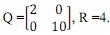

(2C) Design the state observer such that the poles are -8 and -7.

(2D) Design the Kalman-Bucy filter with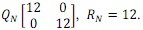

(3). Analyse the performance of the closed-loop system:

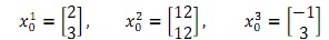
Compare the LQR performance index for the closed-loop system using state feedback (2A) and the closed-loop system using state feedback in (2B). Use the Q and R given in (2B). Compute the value of the performance index of each system for three different initial state values

(4). Assume we want to control the ball position to 0.5 instead of 0, design the state feedback set point control law with the poles of the closed-loop to be -6 and -7.

Question 2:

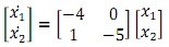
Examine the state space model of the inverted pendulum (Question 1 in Assignment 1),

(1) Write MATLAB code to design a state observer such that the poles of the observer are -5,- 3,-6,-8.

(2) Write MATLAB code to design state feedback control law u=-Kx such that the poles of the closed-loop system are -4, -3, -5, -7 (as in Assignment 1 Question 1). Describe the state- space model of the closed-loop system including the observer and feedback control.

(3) Simulate the state trajectory of both the open-loop system and the closed-loop system (state feedback case only) for any given initial states by Simulink.

Question 3:

Consider system

Choose V(x) = x₁² + 3x₂² and use Lyapunov stability theorem to demonstrate that the equilibrium state of the system is stable.

Question 4:

Consider a mobile robot following a circular trajectory. The mobile robot position at time t is denoted as (x(t), y(t)) and its orientation at time t is denoted as θ(t), the velocity and turn rate are denoted as ??(t) and ??(t) respectively. The nonlinear motion model can be simplified as

Suppose the desired trajectory (reference trajectory) is a circular trajectory

where (x₀, y0) is the center of the circle, and R is the radius of the circle. Then the reference trajectory satisfies

where v_r = Rω_r

Consider the difference between the actual robot trajectory and the desired robot trajectory in the robot local frame. That is, define new state as

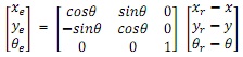
Then the tracking error model is

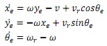
Define the new control as

(1) Derive the nonlinear state space model of the system with state (x_e, y_e, θ_e) and control (v_e, w_e).

(2) Assuming x_e, y_e, θ_e, v_e, ω_e are all close to zero, linearise the system at the operating point (x_e, y_e, θ_e, v_e, w_e) = (0,0,0,0,0) to derive the state-space model of the linearised control system.

(3) Let v_r = 0.6, w_r = 30°. Design state feedback control law for the linearised system such that the poles of the closed loop system are -4,-6,-10.

(4) Let v_r = 0.5, w_r = 30°. Design the state feedback LQR control for the linearised system with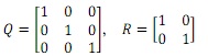

Question 5:

Use MATLAB simulator or Simulink to test the controller design using the model developed in Question 4 (set the desired velocity as 0.6 and the desired turn rate as 30°). A template of the MATLAB simulator and a Simulink model are provided which is used to simulate a robot moving along a straight line. You are required to

(1) change the simulator or Simulink to be the circular trajectory situation and complete the open-loop (simply fix the velocity and turn rate) and closed-loop control design (using pole placement and LQR on the linearised model as in Question 4) and integrate it with the MATLAB simulator or Simulink,

(2) compare the performance of the closed-loop systems using different controllers with that of the open-loop system, and discuss the results obtained.

For MATLAB Simulator, you are suggested to use the following template:
Run Ass2_49329_Simulation_template.m for the simulator. Choose open-loop or closed-loop in line 9-10:
closed_loop=0; % open-loop closed_loop=1; % closed-loop
You can change the simulation time period in line 12: time_period = 100; % simulation time period
For the closed-loop design, you need to modify the file: control_velocity_turnrate_49329.m

For Simulink, you are suggested to use the following template: Mobile_robot_open_loop.slx Mobile_robot_close_loop_with_noises_straight_line.slx