Assets Markets and the LM Curve

The assets markets are the markets in which money, bonds, stocks, houses and other forms of wealth are traded. There are a large variety of assets and a lot of trading takes place in the assets markets everyday. But, we shall simplify matters by grouping all available assets into two groups, money and all other assets. Given the level of financial wealth, an individual who has decided how much to invest in other assets has implicitly also decided how much money to hold. Our focus will be on the money market, which implicitly takes care of the other assets market.

Before proceeding ahead, we need to know the distinction between nominal demand for money and real demand for money. Nominal demand for money is the individual's demand for a given number of rupees. Whereas, real demand for money is the demand for money expressed in terms of the number of units of goods that money will buy; it is equal to the nominal demand for money divided by the price level. Similarly, real money balances are the quantity of nominal money divided by the price level.

We turn now to demand for money. The demand for money is a demand for real money balances - real balances for short - because people hold money for what it will buy. The higher the price level, the more nominal balances a person has to hold to be able to purchase a given quantity of goods. If the price level doubles, then an individual has to hold twice as many nominal balances in order to be able to buy the same amount of goods. What are the determinants of demand for real balances? They are level of real income and the interest rate. It depends on the level of real income because individuals hold money to pay for their purchases, which in turn, depend on income. The demand for money depends also on the cost of holding money. The cost of holding money is the interest that is forgone by holding money rather than other assets. For our analysis, we take the demand for real balances to be

L = kY  -  hi ;     k, h > 0

The parameters k and h reflect the sensitivity of the demand for real balances to the level of income and the interest rate.

Now we proceed to the derivation of the LM Curve. Assume the nominal quantity of money to be   . We assume the price level is constant at the level     so that the real supply of money is at the level   .

For equilibrium in the money market, the supply of real money should be equal to the demand for real money balances.

Figure 1

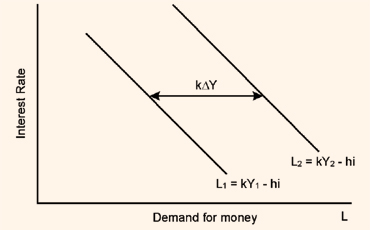
The demand for real money balances is shown in figure 5.4. The demand schedule L₁ is for a particular income level Y₁. The income is held constant but the interest rate is varied to see what the demand for real balances is. This exercise gives the demand schedule L₁. A similar exercise is done for a higher level of income Y₂ and we get the schedule L₂.

The demand schedule L₂ is to the right of L₁ because for a given interest rate, the demand for money increases with the increase in the level of income. The increase in demand for real balances would be equal to  KΔY  . This is shown in figure 5.4.

Figure 2

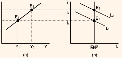
Now, let us see how we can draw the LM Curve. Suppose the real money supply is fixed at    as shown by the vertical line in Figure 5.5(b). If the level of income is Y₁, the demand for real balances for various rates of interest is shown by the line L₁. The point E₁, where the demand for money schedule cuts the vertical line showing the supply of money, indicates that demand for real balances is equal to the supply of real balances. The income and interest rate corresponding to the point E₁ are Y₁ and i₁ (shown on the vertical axis). Y₁ and i₁ are plotted in figure 5.5(a) to give the point E₁. A similar exercise is done for a higher level of income Y₂ and we get the point E₂. Combining the points E₁, E₂, etc. in figure 5.5(a), gives us the LM Curve. The LM Curve gives the combinations of income and interest rates which produce equilibrium in the money market. For all points on the LM Curve, the demand for real balances is equal to supply of real balances.

The equation of the LM Curve can be derived as follows:

For equilibrium in the money market, the demand for real balances is equal to supply of real balances. Thus

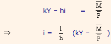
The above relationship is the equation of the LM Curve. From this equation we see that the greater the responsiveness of the demand for money to income, as

measured by k, and the lower the responsiveness of the demand for money to the interest rate, h, the steeper is the LM Curve.

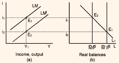
The real money supply is held constant along the LM Curve. Therefore, a change in the real money supply should shift the LM Curve. We can see from the equation of the LM Curve that an increase in real money supply should shift the LM Curve down and to the right whereas a decrease in the real money supply should shift the LM Curve up and to the left.

Figure 3

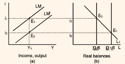
We can also see from figure 5.6 why the LM Curve should shift to the right when there is an increase in the real money supply. The original money supply is   and the corresponding LM Curve is shown by the line marked LM. When the real money supply increases to   , the vertical line showing the supply of money shifts to the right, as shown in the figure. Now the equilibrium in the money market is produced at point E2. For the same level of income too, the equilibrium rate of interest will fall. Thus, we get a new LM Curve which is below the original LM Curve.

Points on the LM curve indicate a situation of the supply of money being equal to the demand for money. What do points which do not lie on the LM Curve indicate? Do they indicate excess demand for money or excess supply of money?

Figure 4

In figure 4, point E1shows the equilibrium in the money market for income level Y1. If there is an increase in income to Y₂, the demand for real balances will rise as indicated by the Curve L₂. At the initial interest rate i₁, the demand for real balances would be indicated by point E₄ in figure 4, and we would have an excess demand for money equal to the distance E₁E₄. Accordingly, point E₄ in figure 4 is a point of excess demand for money.

A similar reasoning shows that at point E₃there is an excess supply of money. More generally, any point to the right and below the LM schedule is a point of excess demand for money, and any point to the left and above the LM Curve is a point of excess supply.