Reference no: EM132188078

Question (1): Let A ∈ R^(n+m)×(n+m) be symmetric positive definite, with

A =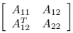 

where A₁₁ ∈ R^n×n, A₁₂ ∈ R^n×m, A₂₂ ∈ R^m×m, and let L be the cholesky factor of A, A = LL^T. Partition L as

L = 

where L₁₁ ∈ R^n×n, L₂₁ ∈ R^n×m, L₂₂ ∈ R^m×m.

(a) Show that L₂₂L^T₂₂ = S where S = A₂₂ - A^T₁₂A^-1₁₂ is the Schur complement of A₁₁ in A.

(b) Using the foregoing relations to drive a block version of the Cholesky factorization algorithm. Note that the algorithm should not require any explicit matrix inversion.

Question (2): Linear systems that arise in many applications can become quite large. It is often necessary to exploit any structure and /or sparsity in the matrices to reduce the computation burden. We will consider the one-dimensional Poisson equation: -y''(t) = f(t) on [0,1], with y(0) = y(1) = 0.

Such problems are frequently very hard to handle because it is often not possible to express y(t) in terms of elementary functions (as is done in undergraduate courses on ODE). Numerical methods are employed in order to approximate y(t) at discrete points inside the interval [a,b]. This approach will leads to a linear system of equations (we will learn how in the numerical PDE class).

The approach we consider begins by subdividing the interval [a,b] into n + 1 equal subintervals, each of length b-a/n+1: t₀ = a, t₁ = a + h, t₂ = a + 2h, ......, t_n = a + nh, t_n+1 = b; The points t_i = a + ih are called grid points, and the value h = b-a/n+1 is called the step size. Smaller step sizes generally produce better approximations to the derivatives, so better accuracy requires smaller step size, and hence larger number of grid points. Let yi = y(t_i) and f_i = f (t_i), and show that by using the finite difference method, we can compute approximations to yi by solving the linear system T_y = h²f , where

T =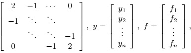 

(a) Prove that the matrix T has an LU factorization with L(i, i) = 1 and L(i + 1, i) = -i/i+1 , U (i, i) = i+1/i and U (i, i + 1) = -1.

(b) Is partial pivoting needed?

(c) Write a Matlab function T = poissonmat(n) which created the n × n matrix T for given n.

(d) Write a Matlab function y = poissonsolve(f ) which, given a vector f of length n, computes the solution y of T y = h²f .

(e) Let f (t) = sinΠt, then the right hand side f_i = sinΠ(t_i). Experiment with various values of n, say n = 10, 100, 500, 1000. Fill the following table:

Question (3): We consider the approximations to the eigenvalues and eigenfunctions of the one-dimensional Laplace Operator L[u] = -d²u/dx² on the unit interval [0,1] with boundary u(0) = u(1) = 0. A scalar λ is an eigenvalue of L if there exists a twice -differentiable function u s. t. -u''(x) = λu(x) on [0,1] with u(0) = u(1) = 0. In this case u is said to be an eigenfunction of L corresponding to the eigenvalue λ. This continuous problem can be approximated by the discrete eigenvalue problem

where we have set

T =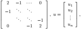

with u_i = u(x_i). It can be shown that the N × N matrix TN has eigen-values ν_j = 2(1 - cosΠj/N+1) for j = 1 : N, corresponding to the eigenvectors u_j(k) = √2/(N+1) sin(jkΠ)/(N+1) is the kth entry in u_j. Notice that the eigenvec-tors are normalized w.r.t. the 2-norm. Also notice that eigenvalues of T_n lie in the interval (0,4). Hence, the eigenvalues of h^-2TN lie in the interval (0, 4(N + 1)²).

(a) Express the spectral condition number κ = λ_N /λ₁ of T_N (which is the same as the condition number of h-2TN ) as a simple function of N for N → ∞.

(b) Use Matlab to plot the eigenvalues of T_N for N = 21 (from smallest to largest).

(c) Again using N = 21, use Matlab to plot the eigenvectors u_j of T_N for j = 1, 2, 3, 5, 11, 21. The plot should be of the form (k, u_j(k)) where k = 1 : 21. Note that as j increases, the behavior of the eigenvectors (approximate eigenfunctions) becomes increasingly oscil- latory;these eigenfunctions are often called "high energy modes".

(d) Write a Matlab code implementing the power method to compute approximations of the largest eigenvalue λ_N of L and corresponding eigenfunctions. Use N = 500 and apply the algorithm to h^-2TN . Start with a random initial guess, use normalization in the 2-norm, and stope when the difference of two subsequent approximate eigenvectors has 2-norm less than some prescribed tolerance τ . (e. g. τ = 10^-6).
(i) Report the number of iterations performed
(ii) compared approximations with exact eigenvalue/eigenvector pair.
(iii) Use matalb to plot the computed eigenvector.

(e) Write a Matlab code implementing the inverse power method to compute approximations of the smallest eigenvalue λ₁ = π² of L and cor- responding eigenfunctions. Use N = 500 and apply the algorithm to h^-2TN . Start with a random initial guess, use normalization in the 2-norm, and stope when the difference of two subsequent approximate eigenvectors has 2-norm less than some prescribed tolerance τ . (e. g. τ = 10^-6).
(i) Report the number of iterations performed
(ii) compared approximations with exact eigenvalue/eigenvector pair.
(iii) Use matalb to plot the computed eigenvector.

Question (4): Use the poisson3d.m code to build linear systems A_u = b. In the Matlab scripts you will have three linear systems which are the dis- cretizations of the Poisson's equation in 1, 2, and 3 dimension.
- We will consider the conjugate gradient methods with preconditioners.
- Increase the size of m in the code, which is the grid size for the dis- cretization. Run pcg again, and find the iteration numbers.
- set the stopping tolerance 10^-12.
- You can use help or doc to find the syntax of pcg.
- Preconditioner P₁: we can consider to use the incomplete Cholesky fac- torizations. (in Matlab ichol). L = ichol(K3D, struct(′type′,′ ict′,′ droptol′, 1e^-02,′ michol′,′ of f ′)), we set P₁ = L^T∗L as our preconditioner.
- Another preconditioner P₂: we can consider is the diagonal matrix of A. P₂ = diag(diag(A))
- Or we can use the preconditioner P₃, here P₃ = triu(A);
- Compare the three preconditioners for each dimensional case, and re- port the best preconditioner you choose. Here are some key points you need to include in your report:

(a) For n = 1, this is the Poisson in 1D case. Report the iteration numbers for the following:

(b) Repeat your tests for the poisson in 2D and 3D. Report the iteration numbers;

(c) For each dimension, plot the computed solutions by direct method(backslash in Matlab) and computed solutions by iterative method (pcg).

Choose the best preconditioner you find.

(d) Organize your numerical data, report them by tables or figures.

(e) Don't forget to report what you have observed and your conclusions.