Euler's Method

Up to this point practically all differential equations which we've been presented along with could be solved. The problem along with this is which the exceptions quite than the rule are. The vast majority of first order differential equations can't be solved.

So as to teach you something about solving first order differential equations we've had to control ourselves down to the rather restrictive cases of separable, linear or exact differential equations or differential equations which could be solved along with a set of very specific substitutions. Most first order differential equations though fall in none of these categories. Actually even those that are separable or accurate cannot always be solved for an explicit solution. Without explicit solutions to such this would be hard to find any information about the solution.

Therefore what do we do when faced along with a differential equation which we can't solve? The answer based on what you are looking for. If you are merely looking for long term behavior of a solution you can always draw a direction field. It can be done without too much difficulty for some fairly complicated differential equations which we can't solve to find exact solutions.

The problem with this approach is which it's only actually good for getting common trends in solutions and for long term behavior of solutions. There are times while we will require something more. For illustration, maybe we need to find out how an exact solution behaves, including some values as the solution will take. There are also a quite large set of differential equations which are not easy to sketch good direction fields for.

In these cases we resort to numerical methods which will permit us to approximate solutions to differential equations. There are several different methods which can be used to approximate solutions to a differential equation and actually whole classes can be taught just dealing with the different methods. We are going to look at one of the oldest and simplest to use here. This method was initially devised through Euler and is termed as, oddly adequate, Euler's Method.

Here we start with a general first order IVP,

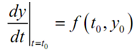
dy/dt = f(t,y),   y(t₀) = y₀   .........................(1)

Here f(t,y) is a identified function and the values in the initial condition are also identified numbers. From the second theorem in the Intervals of Validity section we identify that if f and fy are continuous functions so there is a unique solution to the Initial Value Problem in some interval surrounding t = t₀. Thus, let's suppose that everything is nice and continuous hence we know that a solution will actually exist.

We need to approximate the solution to (1) near t = t₀.  We'll start along with the two pieces of information which we identify about the solution. Firstly, we identify the value of the solution at t = t₀ from the initial condition. Second, we also identify the value of the derivative at t = t₀.  We can find this by plugging the initial condition in f(t,y) in the differential equation itself. Hence, the derivative at that point is,

Here, we notice that these two pieces of information are sufficient for us to write down the equation of the tangent line to the solution on t = t₀. The tangent line is y = y₀ + f (t₀, y₀) (t --t₀).

See the figure as given below:

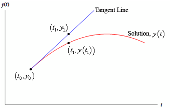
If t₁ is close adequate to t₀ so the point y₁ on the tangent line must be fairly close to the actual value of the solution at t₁, or y(t₁). Determining y₁ is easy sufficient. All we require to do is plug t₁ in the equation for the tangent line.

y₁ = y₀ + f (t₀ , y₀)( t₁ - t₀)

Here, we would like to proceed in a same manner, but we don't contain the value of the solution at t₁ and so we won't identify the slope of the tangent line to the solution at such point. It is a problem. We can partially resolve it though, by recalling which y₁ is an approximation to the solution at t₁. If y₁ is an extremely good approximation to the actual value of the solution so we can use which to estimate the slope of the tangent line at t₁.

Thus, let's hope that y₁ is a superior approximation to the solution and construct a line by the point (t₁, y₁) that has slope f (t₁, y₁). This provides:

y = y₁ + f (t₁ , y₁) (t - t₁ )

Here, to find an approximation to the solution at t = t₂ we will expect that such new line will be quite close to the actual solution at t₂ and utilize the value of the line at t₂ as an approximation to the actual solution. This provides.

y₂  = y₁ + f (t₁ , y₁ ) (t₂  - t₁ )

We can continue in this style. Utilize the previously computed approximation to find the next approximation. Then,

y₃  = y₂ + f (t₂ , y₂ ) (t₃  - t₂)

y₄  = y₃ + f (t₃ , y₃ ) (t₄  - t₃)

And so on.

Generally, if we have t_n and the approximation to the solution at such point, y_n, and we need to get the approximation at t_n+1 all we require to do is use the subsequent.

Y_n+1 = y_n + f (t_n , y_n ) ⋅ (t_n+1  - t_n)

If we describe

 f_n  =  f (t_n , y_n ) we can simplify the formula to

y_{n +1} = y_n + f_n ⋅ (t_{n +1} - t_n )   .....................(2)

Frequently, we will suppose that the step sizes among the points t₀ , t₁ , t₂ , ... are of a uniform size of h.  Conversely, we will frequently assume as

t_{n +1} - t_n = h

This doesn't have to be done and there are times when it's best that we not do this. However, if we do the formula for the next approximation becomes.

 y_{n +1} = y_n + h f_n   ............(3)

Thus, how do we use Euler's Method?  It's quite simple.  We begin with (1) and then decide if we need to use a uniform step size or not. So starting with (t₀, y₀) we repeatedly evaluate (2) or (3) depending on whether we decided to use a uniform set size or not. We carry on until we've gone the decided number of steps or reached the decided time.  This will provide us a sequence of numbers y₁ , y₂ , y₃ , ... y_n   which will approximate the value of the actual solution at t₁ , t₂ , t₃ , ... t_n.

What do we do if we need a value of the solution at several other points than those used here? One opportunity is to go back and again describe our set of points to a new set which will comprise the points we are after and redo Euler's Method using this new set of points.  Though this is cumbersome and could take much time especially if we had to make changes to the set of points more than one time.

The other possibility is to remember how we reach the approximations in the first place. Recall which we used the tangent line,

y = y₀ + f (t₀ , y₀ ) (t - t₀ ) to find the value of y₁. We could utilize this tangent line as an approximation for the solution on the interval [t₀, t₁]. Similarly, we used the tangent line

y = y₁ + f (t₁ , y₁ )( t - t₁) to find the value of y₂. We could utilize this tangent line as an approximation for the solution on the interval [t₁, t₂]. Continuing in this way we would find a set of lines that, while strung together, must be an approximation to the solution as an entire.

In practice you would require to write a computer program to do such computations for you. Mostly in cases the function f(t,y) would be more large or/and complicated to utilize by hand and in most serious uses of Euler's Method you would need to utilize hundreds of steps that would make doing this through hand prohibitive. Thus, here is a bit of pseudo-code which you can use to write a program for Euler's Method which uses a uniform step size, h.

1.   Define f (t, y).

 2.   input t₀ and y₀.

3.   input step size, h and the number of steps, n.

4.   for j from 1 to n do a.       m = f (t₀, y₀) b.    y₁  = y₀ + h*m c.       t₁  = t₀ + h

d.   Print t₁ and y₁

e. t₀ = t₁

f. y₀ = y₁

5.   end

The pseudo-code for a non-uniform step size would be some more complicated, however it would fundamentally be similar.

Therefore, let's take a look at a couple of illustrations. We'll utilize Euler's Method to approximate solutions to a couple of first order differential equations. The differential equations which we'll be using are linear first order differential equations which can be easily solved for an exact solution. Certainly, in practice we wouldn't use Euler's Method on such kinds of differential equations, although by using simply solvable differential equations we will be capable to verify the accuracy of the method. Identifying the accuracy of any approximation method is a fine thing.  It is significant to know if the method is liable to provide a superior approximation or not.