Reference no: EM131038360
Intermediate Applied Statistics for Education
Question 1- 100 SLU students were polled and asked both their GPA and the number of hours per week they watch TV. Among them were four students named Karen, Tara, Katyn, and Nicole. Below is a scatterplot of GPA against the number of hours watched.

(a) Fill in the following table with "small" or "large" in each box.
|
|
Residual
|
Leverage
|
Influence
|
|
Karen
|
|
|
|
|
Tara
|
|
|
|
|
Katyn
|
|
|
|
|
Nicole
|
|
|
|
(b) If you ran the regression of GPA on hours watched omitting whichever of the 4 points above you deemed most influential, what do you expect would happen to the slope coefficient?
(c) Should you remove this point from the analysis? Why or why not? Explain what factors you would consider in determining whether you should.
Question 2- Katyn runs a regression of Y on X and obtains an R2 value of exactly 0.00. Katyn says, "I get it! That means there is no relationship between Y and X in this sample!" Nicole, sitting in the next office, comes running in and asks Katyn to generate a scatterplot of Y against X. Once they saw the scatterplot (above), it was clear to everyone that Katyn's claim was way off.
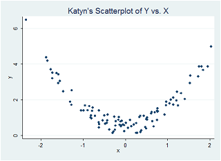
(a) Explain why Katyn's claim was incorrect.
(b) What type of bias did the model suffer from (choose one):
a. Simultaneous causality bias
b. Model misspecification bias
c. Sample selection bias
d. Bias due to measurement errorinX
e. Both (a) and (d)
(c) Posit a model to reflect the relationship you observe. Write out the statistical model in equation form.
Question 3- The following series of models test the relationship between "happiness" (as measured in "happiness units" on a continuous scale) and various predictors, including the personal income of the individual, an indicator for whether the individual has completed a PhD degree (PhD degree completed = 1, no PhD degree = 0), and an indicator for whether the person is a SLU graduate (SLU graduate = 1, not a graduate of SLU = 0). The sample is a sample of adults holding at least a bachelor's degree (or more). Results from 5 different models are presented below.
Regression models predicting happiness
|
|
Model 1
|
Model 2
|
Model 3
|
Model 4
|
Model 5
|
|
|
|
|
|
|
|
|
PhD degree
(indicator variable)
|
0.86**
|
6.86***
|
6.86***
|
6.86***
|
6.86***
|
|
(0.38)
|
(0.18)
|
(0.18)
|
(0.18)
|
(0.18)
|
|
SLU graduate
(indicator variable)
|
5.47***
|
3.16***
|
3.15***
|
3.15***
|
3.16***
|
|
(0.27)
|
(0.18)
|
(0.18)
|
(0.18)
|
(0.18)
|
|
Income
|
|
0.44***
|
2.07**
|
-17.91
|
|
|
|
|
(0.03)
|
(0.72)
|
(13.09)
|
|
|
Income2
|
|
|
-0.03*
|
0.65
|
|
|
|
|
|
(0.01)
|
(0.44)
|
|
|
Income3
|
|
|
|
-0.008
|
|
|
|
|
|
|
(0.005)
|
|
|
Ln(income)
|
|
|
|
|
12.99***
|
|
|
|
|
|
|
(1.90)
|
|
Constant
|
3.32***
|
1.88*
|
-22.01*
|
172.51
|
-29.06***
|
|
|
(1.00)
|
(0.92)
|
(10.53)
|
(127.66)
|
(3.05)
|
|
|
|
|
|
|
|
|
Adjusted R-squared
|
0.02
|
0.19
|
0.20
|
0.20
|
0.16
|
|
N
|
7986
|
7986
|
7986
|
7986
|
7986
|
|
Significance levels: * p<0.05, ** p<0.01, *** p<0.001
|
(a) Interpret the following coefficients (explain in substantive terms what these coefficients mean):
i. Intercept in model 1
ii. PhD degree in model 1
iii. SLU Graduate in model 1
iv. PhD degree in model 2
v. SLU Graduate in model 2
vi. Income in model 2
vii. Ln(Income) in model 5
(b) Say which of the modelsabove you would choose and why. Make a compelling argument, and make reference to each of the models (i.e., compare the relevant attributes of the models, and explain why the one you prefer is preferable to the others).
Model 4, by looking to the Adjusted R-squared 0.20 and constant 172.51 (127.66), model 4 has the highest number.
(c) Write the equation of the fitted model for Model 5. Happiness =0.86+-.02(income)+-3.16(income)2+.12.99(income)3
(d) Consider the null hypothesis that the true coefficient on PhD degree is equal to 7.0 in model 2.
i. In plain English (i.e., in the real world), what does this null hypothesis correspond to? (Do not use the word "slope" in your answer.)
ii. Calculate a t-statistic to test this null hypothesis.
iii. Based on the t-statistic for this null hypothesis, what do you conclude?
(e) Construct a 95% confidence interval for the slope on SLU Graduate from Model 2. Carefully and precisely interpret the meaning of the confidence interval. (Include the word "95%" in your interpretation.)
(f) Is there evidence that omitting Income from Model 2 led the estimate on SLU Graduate (in Model 1) to be biased? How did you determine this? Provide a plausible explanation for why this estimate is or is not biased.
(g) One more model is fit using these data. This model includes an interaction term between the PhD and SLU Graduate variables (the product of these two variables). In this new model, the estimated coefficient on PhD is 0.30 (standard error=0.21; p-value=0.16); the estimated coefficient on SLU Graduate is 2.90 (standard error=0.22; p-value<0.001); and the estimated coefficient on the interaction term is 12.50 (standard error=0.46; p-value<.001). The coefficient(s) on the income variables is/are the same as those in the model you selected in (b) above.
i. Based on these results, if you met two non-SLU graduates (UMSL graduates, for example), each making the same income, one of whom had a PhD and one of whom had a BA degree, how much happier/sadder would you predict the PhD recipient is than the BA recipient? Explain whether you can reject the hypothesis that, in fact, non-SLU PhD recipients are equally as happy/sad as non-SLU BA recipients.
ii. How much happier, on average, are SLU PhD recipients than UMSL (or other non-SLU) PhD recipients earning the same income? How would you test whether this difference is statistically significant? (You don't have to do the test, just state the null hypothesis and show how you would test it in Stata.)
Question 4- Nicole and Karen are presenting new research on variation between counties in school size (school enrollment). In their paper (entitled "School enrollment does not vary by county"), they use data on a sample of schools in California and run a simple univariate regression of total school enrollment (variable name: enrl_tot) on county code (variable name: cntycode). County code is constructed as the alphabetical order of counties (e.g, Alameda county has a cntycode of 1, Butte county has a cntycode of 2, etc.; there are 45 counties represented in their data). The Stata output from Nicole and Karen's model is:
. reg enrl_tot cntycode
Source | SS df MS Number of obs = 420
-------------+------------------------------ F( 1, 418) = 0.05
Model | 706239.418 1 706239.418 Prob > F = 0.8302
Residual | 6.4152e+09 418 15347333.6 R-squared = 0.0001
-------------+------------------------------ Adj R-squared = -0.0023
Total | 6.4159e+09 419 15312390.6 Root MSE = 3917.6
------------------------------------------------------------------------------
enrl_tot | Coef. Std. Err. t P>|t| [95% Conf. Interval]
-------------+----------------------------------------------------------------
cntycode | -3.349142 15.61256 -0.21 0.830 -34.03805 27.33977
_cons | 2710.799 427.4141 6.34 0.000 1870.65 3550.948
------------------------------------------------------------------------------
Nicole and Karen notice the p-value on their omnibus F-test is 0.8302, so they conclude that school enrollment does not vary by county.
As luck would have it, Katyn and Tara used the same dataset and are presenting at the same conference (in fact, at the very same panel) their own paper entitled "School enrollment varies by county." In their paper, Katyn and Tara included indicator variables for each county (excluding Alameda County). The p¬-value on the omnibus F-test for Katyn and Tara's model is extremely small (<0.001), leading them to conclude that school enrollment varies significantly across counties. The Stata output from Katyn and Tara's model is:
. reg enrl_tot county2-county45
Source | SS df MS Number of obs = 420
-------------+------------------------------ F( 44, 375) = 3.87
Model | 2.0041e+09 44 45548592.5 Prob > F = 0.0000
Residual | 4.4118e+09 375 11764676.3 R-squared = 0.3124
-------------+------------------------------ Adj R-squared = 0.2317
Total | 6.4159e+09 419 15312390.6 Root MSE = 3430
------------------------------------------------------------------------------
enrl_tot | Coef. Std. Err. t P>|t| [95% Conf. Interval]
------------- +----------------------------------------------------------------
county2 | 957.5 3704.788 0.26 0.796 -6327.263 8242.263
county3 | 582 4850.706 0.12 0.905 -8955.993 10119.99
county4 | 2530.857 3666.789 0.69 0.490 -4679.188 9740.902
. | . . . . . .
. | . . . . . .
. | . . . . . .
county44 | 4432.778 3615.503 1.23 0.221 -2676.423 11541.98
county45 | 744.5 4200.835 0.18 0.859 -7515.644 9004.644
_cons | 195 3429.967 0.06 0.955 -6549.38 6939.38
------------- +----------------------------------------------------------------
(a) Which paper-Nicole and Karen's or Katyn and Tara's -has a better analysis to address the question of whether total district enrollment varies by county in California? What makes this analysis better?
(b) Why did Katyn and Tara omit the indicator variable for Alameda County (i.e. county1) from their list of regressors?
(c) Based on the regression output from Katyn and Tara's paper, what would you predict would be the enrollment of an average school in Butte County (county2)?