Reference no: EM132293496

Project 1: Heat Transfer from Extended Surfaces

Problem Description - The problem of electronics cooling remains a challenge that engineers are facing while designing electronic components. The use of fins is one of the basic inexpensive solutions to increase the rate of heat transfer from a hot surface to the surrounding fluid. The main objective of this assessment is to simulate the heat transfer and temperature distribution from an single pin fin for different tip boundary conditions and compare the results to the analytical solutions available in the literature.

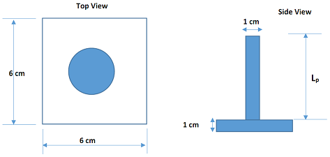
Case I: A pin fin made of Aluminum is attached to a hot surface with a side length of 6 cm (see figure below). The pin fin diameter and length are D_p = 10 mm and L_p = 30 cm. The surface temperature of the hot chip is 75^oC when the system is in ambient air temperature of 25^oC, and the convection coefficient is 250 W/m².K. The thermal conductivity of the used Aluminum is 177 W/m.K.

CFD Analysis using Fluent -

1. Perform a CFD analysis of the geometry described above assuming that the chip is at uniform temperature of 75^oC and that it is made of the same material as the fins.

2. Three fin tip boundary conditions have to be studied:

a) Adiabatic fin tip.

b) Convective fin tip.

c) Prescribed tip temperature: T= 35^oC.

3. Required CFD results are: temperature contours and total heat transfer rate from the chip

4. Plot the variation of the temperature along the fin.

Analytical Solution -

1. The temperature distribution along a fin is derived in most transfer books. Apply the resulting analytical solution of the temperature distribution along the fin to the simulation solution and discuss any discrepancy between the results.

2. Calculate the total heat flux from the chip analytically and compare it to the CFD report of total heat transfer rate.

Submit a concise report (not exceeding 1500 words) and including:

• A brief discussion of the methods used in the simulation
• Sketches, diagrams, pictures the required plots, contours...
• Comparison of the temperature distribution for all 3 boundary conditions.
• Discussion of the accuracy of CFD results and possible reasons for the discrepancies between the simulation results analytical solutions.

Project 2: Simulation of the Flow in a Double Pipe Heat Exchanger

Problem Description - Heat exchangers are devices used to transfer heat between two fluids. They are commonly used in many systems involving cooling or heating processes, such as powerplants, HVAC systems, automotive systems.... Heat exchangers have many configurations/types: Shell and tube, plate and frame, double pipe...

The main aim of this assessment is to simulate the flow in a double pipe heat exchanger and compare the obtained results to those generated by the well-known effectiveness-NTU methods for heat exchanger analysis.

Case I (Seady-State) - A double-pipe heat exchanger is the simplest type of heat exchangers and easiest to manufacture. It consists of two concentric tubes. The flow arrangement is usually counter-current, since it provides higher heat transfer rate compared to the parallel flow configuration. The cold fluid is placed in the inner tube. It flows at a rate of 0.2 kg/s and its inlet temperature is 30^oC. The hot fluid flows through the annulus with a flow rate of 0.2 kg/s and an inlet temperature of 100^oC. The geometric specifications of the heat exchanger and the properties of the hot and cold fluids are presented in tables 1 and 2.

Table 1: Properties of the hot and cold fluids

Fluid	Hot	Cold
Density (kg/m3)	840	998
Specific Heat (J/kg.K)	2206	4180
Thermal Conductivity (W/m.K)	0.1343	0.616
Viscosity (kg/m.s)	0.1917	0.0007999

Table 2: Geometric specifications of the heat exchanger

Inner Tube Radius (mm)	25
Inner Tube Thickness (mm)	1
Outer Tube Radius (mm)	45
Inner tube Material	Copper
Heat Exchanger Length (mm)	500

CFD Analysis using Fluent -

1. Perform a steady-state CFD analysis of the geometry described above.

2. Required CFD results are: temperature contours and total heat transfer rate between the fluids.

3. Plot the variation of the temperature along the centerline of each fluid.

Analytical Solution -

1. The effectiveness-NTU method is a very popular analysis method to determine the resulting outlet temperature for both fluids in a heat exchanger. Using this method, calculate the outlet temperatures of the hot and cold fluids and the total heat transfer rate between the 2 fluids

2. Compare your results to the solution obtained using Ansys.

Case II (Transient Analysis):

Consider the same heat exchanger geometry. Perform a transient CFD simulation of the flow in the heat exchanger.

Plot the variation of fluid exit temperatures as a function of flow time and comment on the time required to reach steady-state.

Develop and animation of the temperature contours variation with time (not less than 30 seconds).

Submit a concise report (not exceeding 1500 words) and including:

• a brief discussion of the methods used in the simulation (omit unnecessary details)
• sketches, diagrams, pictures the required plots, contours...
• comparison of the fluid exit temperatures using CFD simulations and the analytical solutions.
• discussion of the accuracy of CFD results and possible reasons for the discrepancies between the simulation results of case I and analytical solution

Submit the animation video developed in the transient simulation.