Reference no: EM132873942

Description of coursework

If you use a random number generator for any of the problems below, seed the generator so that the results are reproducible.

Problem 1. Explain and discuss the relevance of the Normal distribution in the context of Monte Carlo estimation.

Problem 2. Consider the function f : R → R given by

f(x) = { (λe^-λx)/e^-λ - e^-2λ if x ∈ [1, 2],

f(x) = {0, otherwise,

for some flied λ > D.

1. Prove that f is a probability density function.

2. Explain how you can generate a sample from f -using the inverse transform method. Implement the inverse transform. method for generating a sample from f in Python and show a histogram of a sample generated from f.

3. Suppose you would like to generate a sample from f using von Neurraann's acceptance-rejection algorithm,

(a) Specify two different prob-ability density functions g1 ≠ g2 with g1 ≠ f and g2 ≠ f that can be used for this purpose. Discuss which of the two pdfs g1 and g2 you prefer to use in von Neumann's acceptance rejection algorithm for generating a sample from f and give reasons for your, choice.

(b) Write down von Neumann's acceptance-rejection algorithm that is designed such. that it has the highest possible acceptance rate for your preferred choice of gb. Explain how you can generate the required sample from. your preferred gi.

(c) Implement von Neumann's acceptance-rejection method for generating a sample from f by using your preferred choice of gi in Python and show a histogram of a sample generated from f .

4. What is your preferred method for generating a sample from f and why?

Problem 3. Consider the standard Black-Scholes financial market consisting of two assets: The riskless asset has time-t price B_t = e^rt, where r ≥ 0 is the constant interest rate and the stock has time-t price

(1) S_t = S₀ exp ((r - σ²/2)t + σw_t)

where S₀ > 0 is the initial stock price, σ > 0 is the volatility., (W_t)t≥o is a standard one-dimensional Brownian motion under the risk-neutruI measure.

Consider an option whose payoff at maturity T > 0 is given by H(S_T), where

H(S_T) = 0,         if S_T ≤ 100,

H(S_T) = 2S_T - 200,         if 100 ≤ S_T ≤ 150,

H(S_T) = 0.25S_T + 62.5,         if 150 ≤ S_T ≤ 350,

H(S_T) = 150,         if S_T ≥ 350,

1. Write down a Monte Carlo estimator together with an asbrmptotic 95% confidence interval for the time-a price of an option with payoff H(S_T) given in 49 and justify your answer. Implement the Monte Carlo estimator and an asymptotic 95% confidence internal for the time-O price of the option with payoff in Python.

2. Specify two alternative estimators for the time-O price of an option with payoff H(ST) that have lower variances than the Monte Carlo estimator considered in part 1. Implement both in Python and discuss and compare their performance.

3. Consider the following function

k(S₀) = E[e^-rTH(S_T)]
where H (S_T) is given in 2.

(a) Explain how you can numerically approximate the derivative of the function k with respect to S₀ denoted by ks₀(S₀) = ∂k(S₀)/∂S₀, assuming that you can-not evaluate this derivative analytically in the following situations:
i. k(S₀) is known analytically;
ii. k(S₀) is not known analytically.

Justify your answers.

(b) Write Python code that numerically approlirnates the derivative kS₀, for the situation (a)(ii) and plot the approximation of the derivative kS₀, as a function of S₀. Discuss your results. In particular, comment on what the financial interpretation of the derivative S₀ is.

Problem 4. Consider a continuous-time stochastic process (log(S_t)t≥0 whose sample paths are simulated on a discrete-time grid given by the points t_i = ih, i ∈ {0, N} where h > 0 and N ∈ N using the following recursive scheme:

Set A(0) = A0 and S(0) = S₀ for some fired A₀, S₀ > 0.

Then, for n = 0,......N - 1 set

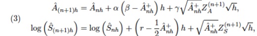
where the 2-dimensional random vectors (Z_A¹. Z_S¹)^T (Z_A^(N), Z_S^(N))^T are and for each n ∈ {0, N - 1} the 2-dimensional random vector (Z_Aⁿ⁺¹ , Z_Sⁿ⁺¹))^T has a multivariate Normal distribution with mean (0,0)^T and covariance matrix 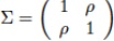where Ρ ∈ (-1, 1).

Furthermore, x⁺= max{x, 0}, log denotes the natural logarithm and α, β, γ ∈ (0, ∞) satisfy 2αβ > γ² and r ≥ 0.

1. Write down. a stochastic differential equation for the stochastic process (log(S_t)) and a stochastic differential equation for a stochastic process (A_t)_t≥0 that can be approximated by the scheme in CV. Justih your answer.

2. Write Python code that implements the simulation scheme given in and use it to plot several realisations of the sample paths of the corresponding stochastic process S.

3. Suppose the scheme in is used to approximate a sample path of (log(S_t)), where (S_t) represents the price of a risky asset (e.g., a stock price). Consider the same option payoff H(S_T) as in Problem 3 a. Write Python code to approximate the time-0 price of this option using a Monte Carlo estimator together with the simulation scheme in a).

Compare your results to the results obtained in the standard Black-Scholes model and discuss your findings.

Attachment:- Computational Finance Assignment.rar