Reference no: EM132567442

Question 1:

Test the claim that the mean GPA of Orange Coast students is larger than the mean GPA of Coastline students at the 0.05 significance level.

The null and alternative hypothesis would be:

The test is:
two-tailed         left-tailed           right-tailed

The sample consisted of 65 Orange Coast students, with a sample mean GPA of 3.32 and a standard deviation of 0.02, and 65 Coastline students, with a sample mean GPA of 3.28 and a standard deviation of 0.06.

The test statistic is:
Thep-value is:
Based on this we:

• Fail to reject the null hypothesis
• Reject the null hypothesis

Question 2:

For each scenario listed on the left, determine whether the scenario represents an Indepenent Samples or Matched pairs situation by placing the appropriate letter in the box provided.

Comparing pain levels of a group receiving a placebo to a group receiving a medicine
Comparing pain levels before and after treatment with magnetic therapy
Comparing the number of speeding tickets received by men to the number received by women
Comparing pre-test scores before training to post-test scores
a. Independent Samples
b. Matched Pairs

Question 3:
A survey of 30 people was conducted to compare their self-reported height to their actual height. The difference between reported height and actual height was calculated.

You're testing the claim that the mean difference is greater than 1.3.

From the sample, the mean difference was 1.35, with a standard deviation of 0.54. Calculate the test statistic, rounded to two decimal places

Question 4:

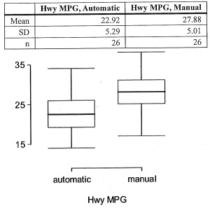
The table provides summary statistics on highway fuel economy of cars manufactured in 2012 (from Exercise 5.32). Use these statistics to calculate a 98% confidence interval for the difference between average highway mileage of manual and automatic cars, and interpret this interval in the context of the data.

lower bound:
upper bound:

Interpret your confidence interval in the context of the problem:

• We can be 98% confident that the difference in average highway mileage of manual and automatic cars is contained within our confidence interval
• 98% of manual and automatic cars will have a difference in highway mileage that falls within our confidence interval
• We can be 98% confident that our confidence interval contains the difference in average highway mileage of the cars in our sample is contained within our confidence interval

Does your confidence interval provide significant evidence for a difference in the highway fuel efficiency of automatic versus manual cars? Explain.

• yes, since 0 is not contained within our confidence interval 0 no, since negative highway mileage doesn't make sense
• yes, since highway mileage cannot be negative
• no, since 0 is not contained within our confidence interval

Question 5:
Two samples are taken with the following sample means, sizes, and standard deviations = 20 = 27
‾x1 = 20 ‾x2 = 27

n1 = 51  n2 = 54

S1 = 5  s2 = 4

Estimate the difference in population means using a 99% confidence level. Use a calculator, and do NOT pool the sample variances. Round answers to the nearest hundredth.

Question 6:

In order for you to use the goodnees-of-fit test, the test of independence, or the test of homogeneity, the expected frequencies for each cell needs to be at least

Question 7:

You intend to conduct a goodness-of-fit test for a multinomial distribution with 6 categories. You collect data from 68 subjects.

What are the degrees of freedom for the x2 distribution for this test? d. f. =

Question 8:

You are conducting a test of independence for the claim that there is an association between the row variable and the column variable.
What is the chi-square test-statistic for this data?

x² =
Report all answers accurate to three decimal places.

Question 9:

You are conducting a test of homogeneity for the claim that two different populations have the same proportions of the following two characteristics. Here is the sample data.

What is the chi-square test-statistic for this data?
X² =

Report all answers accurate to three decimal places.

Question 10:
You are conducting a test of the claim that the row variable and the column variable are dependent in the following contingency table.

Give all answers rounded to 3 places after the decimal point, if necessary.
(a) Enter the expected frequencies below:

(b) What is the chi-square test-statistic for this data? Test Statistic: x²
(c) What is the critical value for this test of independence when using a significance level of a =0.10?
Critical Value: x² =
(d) What is the correct conclusion of this hypothesis test at the 0.10 significance level?

• There is not sufficient evidence to warrant rejection of the claim that the row and column variables are dependent.
• There is not sufficient evidence to support the claim that the row and column variables are dependent.
• There is sufficient evidence to support the claim that the row and column variables are dependent.
• There is sufficient evidence to warrant rejection of the claim that the row and column variables are dependent.

Remember to give all answers rounded to 3 places after the decimal point, if necessary.

Question 11:

A regression was run to determine if there is a relationship between hours of TV watched per day (x) and number of situps a person can do (y).

The results of the regression were:
y=ax+b
a=-1.348

b=34.028

r2=0.970225
r=-0.985

Use this to predict the number of situps a person who watches 5.5 hours of TV can do (to one decimal place)

Question 12:
Based on the data shown below, calculate the correlation coefficient (rounded to three decimal places)

Question 13:

Here is a bivariate data set.

x	y
66.7	83.3
102.7	-18.7
59.3	175.2
48.8	15.7
86.8	40.5
82.8	-41.8
78.6	118.3
77.3	-117.4
75.9	149.8
66.7	69.6
75.5	-6.1

Find the correlation coefficient and report it accurate to three decimal places. r =

What proportion of the variation in y can be explained by the variation in the values of x? Report answer as a percentage accurate to one decimal place. r2

Question 14:

You run a regression analysis on a bivariate set of data (n = 77 ). With x‾ = 76.4 and y‾ = 71.9 , you obtain the regression equation

y = 0.539x - 1.879

with a correlation coefficient of r = 0.964 . You want to predict what value (on average) for the response variable will be obtained from a value of 170 as the explanatory variable,

What is the predicted response value? y
(Report answer accurate to one decimal place.)

Question 15:

Match each scatterplot shown below with one of the four specified correlations.