Reference no: EM132476611

ECE 456 - Embedded Control and Mechatronics - Southern Illinois University

Question 1: The state-space equations for a "hanging" pendulum on a cart as shown in Figure 1 can be obtained by replacing θ with Π -θ and ω with -ω in the state-space equations of an inverted pendulum. The normalized form of these equations (see the class notes on inverted pendulum) is given by

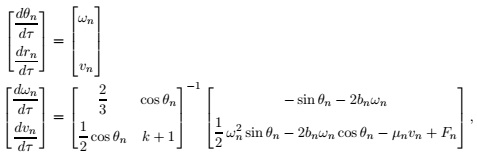
with the normalized parameters

ω₀ = √(g/l), k = M/m, b_n = b/ml²ω₀  µ_n = µ_n/mω₀ .

Figure 1

(i) Set b_n = 0, µ_n = 0, and F_n = 0 and for k = 0, 1, 10 simulate the system starting from the initial state (Π/2, 0, 0, 0). On the same coordinate system, plot each state variable versus Τ for k = 0, 1, 10. Explain your observation.

(ii) Repeat part (a) for b_n = 0, 0.1, 1 and fixed k = 1, µ_n = 0, and F_n = 0.

(iii) Repeat part (a) for µ_n = 0, 0.1, 1 and fixed k = 1, b_n = 0.1, and F_n = 0.

(iv) Simulate the system for k = 1, b_n = 0.1, and µ_n = 1 with the input Fn (Τ ) chosen as a square wave of amplitude 1 and frequencies 0.1, 0.5, 1, 2. Explain your observation.

Question 2: In the liquid-level system of Figure 2, the output valve is always open and the two supply valves are either fully open with the flow rates q_i and q_d, or fully closed. The flow rates of these valves are modeled as q_iu (t) and q_dn (t), where the inputs u (t) and n (t) take only the values of 0 and 1. Assuming that h and qo denote the fluid level and the output flow rate of the tank, the dynamics of the system is given by the state-space equations

dh(t)/dt = -K/C0√h (t) + qi/C0.u (t) + qd/C0 n(t)

qo (t) = K√h(t).

Here, C₀ is the  cross-section of the tank and K is a constant depending on the orifice size of the output valve.

The input n(t) is an uncertain disturbance (it is neither under control nor known to the designer), while u(t) is a control variable. The control goal is to keep the output flow at a constant rate q¯o, or equivalently, to maintain the level of the liquid in the tank at

h¯ = (q¯_o/K)

For this purpose, the following simple feedback law is designed

u (t) =  0, h (t) ≥ h¯

u (t) = 1, h (t) < h¯.

Figure 2

Generate the disturbance n (t) using Bernoulli Binary Generator in Simulink with the Sample time 0.25 and the Probability of a zero 0.5. With the parameter values K = 1, C₀ = 1, q_i = 0.7, q_d = 1, and q₀ = 0.8 (equivalently, h¯ = 0.64) simulate the system starting from the initial state h (0) = 0. Explain your observation and compare two cases in which Probability of a zero is 0.1 and 0.9.

Question 3: In Figure 3, two objects of masses m₁ and m₂ move on a frictionless surface. The objects are connected to each other using a parallel combination of a nonlinear spring and a linear damper of friction coefficient µ, and object 2 is pulled along a line by an external force F . The velocities of the objects are denoted by v₁ and v₂ and their distance is shown by r. The nonlinear spring is at rest when the objects are at a distance r₀, and the force applied by the spring when the objects are at a distance 0 < r < 2r₀ is given by

Φ_s (r) = kr₀ tanh^-1(r/r0 -1), 0 < r < 2r₀,

where k is a constant. Choosing r, v₁, and v₂ as the state variables and F as the input, the state-space equations describing the motion of the objects are expressed as

dr/dt = v₂ - v₁

dv₁/dt = kr₀/m₁ tanh^-1 (r/r₀ - 1) + µ/m₁.(v₂ - v₁)

dv₂/dt = kr₀/m₂ tanh^-1 (r/r₀ - 1) + µ/m₂.(v₁ - v₂) + 1/m₂.F.

Set r₀ = 1, k = 1, and m₂ = 1 and simulate the system under the following assumptions.

In each case explain your observations.

(i) Let µ = 0, m₁ = 1, F = 0, v₁ (0) = v₂ (0) = 0, and r (0) = 1.5, 1.9, 1.99.

(ii) Let µ = 0, F = 0, v₁ (0) = v₂ (0) = 0, r (0) = 1.99, and m₁ = 0.1, 1, 10.

(iii) Let m₁ = 1, F = 0, v₁ (0) = v₂ (0) = 0, r (0) = 1.99, and µ = 0, 0.1, 1.

(iv) Let m₁ = 1, µ = 0.1, v₁ (0) = v₂ (0) = 0, r (0) = 1.99, and assume that F (t) is a step function of the amplitudes 0.5, 1, 1.5.

Figure 3

Question 4: The circuit shown in Figure 4 is a Wien bridge oscillator.

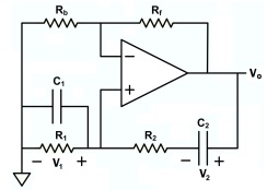
Figure 4

The dynamics of this system is described by the normalized state-space equations

dx₁ (Τ)/dΤ = - (α + 1) x₁ (Τ ) - x₂ (Τ ) + sat (kx₁ (Τ ))

dx2 (Τ)/dΤ = -βx₁ (Τ) - βx₂ (Τ) + βsat (kx₁ (Τ ))

y (Τ ) = sat (kx1 (Τ ))

with the state vector [x₁ (Τ) x₂ (Τ)] and the scalar output y (Τ). The function sat (.) in these equations is the saturation function

sat (z) =  1, z > 1
sat (z) =  z, -1 ≤ z ≤ 1
sat (z) -1, z < -1

and reflects the fact that the output of the operational amplifier saturates at some maximum voltage. The parameters α, β, k, and ω are defined as

α = R₂/R₁, β = C₁/C₂, k = 1 + R_f/R_b, ω = 1/R₂C₁.

For the sake of simplicity, the actual state variables v₁ (t) and v₂ (t) and the actual output v_o (t) are normalized in amplitude to the saturation voltage Vm of the operational amplifier and in time to 1/ω such that in terms of x₁ (Τ ), x₂ (Τ ), and y (Τ ), the voltages v₁ (t) and v₂ (t) of the capacitors C₁ and C₂, and the output v_o (t) of the operational amplifier are given by

v₁ (t) = Vmx₁ (ωt)

v₂ (t) = Vmx₂ (ωt)

v_o (t) = Vmy (ωt) .

Start from the initial state (x₁ (0) , x₂ (0)) = (0.5, 0) and simulate the normalized equations for the following parameter values. For each set of parameter values, plot x₁ (Τ ), x₂ (Τ ), and y (Τ ) versus Τ .

(i) Let α = 1, β = 1, and k = 2, 2.99, 3.01, 3.1, 3.5, 20. Verify that the condition for persistent oscillation is that

k > α + β + 1.

This condition implies that the linearized state-space equations must be unstable. Explain which values of k are reasonable to choose if the goal is to design a sinusoidal oscillator or a rectangular pulse generator.

(ii) Let α = β = 0.1, 1, 10 and k = 1.01(α + β + 1). Explain how the frequency of the oscillator can be adjusted at a desired value.

Question 5: Figure 5 illustrates a simple DC to DC converter. A primary DC source of constant voltage V0 is connected to a resistive load RL via a chopper circuit consisting an electronic switch to turn the circuit on and off, a diode to provide a discharge path for the inductor when the switch is off, and a RLC filter with the resistance RL, the inductance L, and the capacitance C. The electronic switch is controlled by a Pulse Width Modulator (PWM). This modulator turns the switch on and off at a constant frequency ω with a duty cycle 0 ≤ u (t) ≤ 1 (corresponding to the duty cycles of 0% and 100%) regarded as an external control. The combination of the DC source, the electronic switch, and the diode (its voltage drop when turned on is neglected) provides an AC voltage source V0s (t), where s (t) is a binary signal defined as

s (t) = S cos (ωt) - cos (Πu (t))

in terms of the nonlinear function

S (z) = 1, z ≥ 0
S (z) =  0, z < 0.

This AC voltage is filtered by the RLC circuit to deliver an average voltage of V₀u (t) to the load.

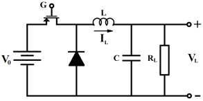
Figure 5

Considering the overall DC to DC converter as a dynamical system with the duty cycle u (t) as its input and the load voltage V_L (t) as its output, the system is described by the nonlinear time-varying

state-space equations

dI_L(t)/dt = - 1/L.V_L(t) + V₀/L.S cos (ωt) - cos (Πu(t))

dV_L(t)/dt = 1/C/I_L(t) - 1/R_LC .V_L (t)

with the state vector consisting the inductor current I_L(t) and the capacitor voltage V_L(t). It is more convenient to use a normalized form of these equations for the purpose of simulations. By introducing the new parameters

 = 1/2√(L/R_L. 1/R_LC), ω₀ = 1/√LC, η = ω/ω₀

the normalized time Τ = ω₀t, and the normalized variables u_n (Τ ), in (Τ ), and v_n (Τ ), the state-space equations (1) are rewritten as

di_n(Τ)/dΤ = - 1/2ζ.v_n (Τ) + 1/2ζ .S cos (ηΤ ) - cos (Πu_n (Τ ))

dv_n (Τ )/dΤ = 2ζi_n (Τ ) - 2ζv_n(Τ ) .

The original unnormalized variables can be determined in terms of their normalized counterparts as

u (t) = u_n (ω₀t)

I_L(t) = V₀/R_Li_n (ω₀t)

V_L (t) = V₀v_n (ω₀t)

Note that the normalized equations (3) depend on only 2 parameters versus 5 parameters for the unnormalized equations (1). Further, the parameters in the normalized equations have a straight- forward representation: ζ is the damping ratio of the RLC filter and η compares the switching frequency with the bandwidth of this filter.

(i) Verify that the unnormalized variables u (t), I_L (t), and V_L (t) as defined by (4), the normalized state-space equations (3), and with the parameters (2), satisfy the state-space equations (1).

(ii) Simulate the normalized state-space equations with the initial state (i_n (0) , v_n (0)) = (0, 0) and the control input (λ is a positive constant)
u_n (Τ ) = 0.5 + 0.5 cos (λΤ ) . (5)

Set η = 10 and ζ = 0.7 and compare the output v_n (Τ ) with the input un (Τ ) for λ = 0.1, 1, 10. Plot un (Τ ), v_n (Τ ), and

s_n (Τ ) = S.cos (ηΤ ) - cos (Πu_n (Τ ))

on the same screen and explain your observation.

(iii) Use the function

u_n (Τ ) = 0.3, 0 ≤ Τ < 10
u_n (Τ ) = 0.7, Τ ≥ 10

as the input and repeat part (b) by setting η = 10 and changing the damping ratio for the values ζ = 0.2, 0.4, 0.7, 1, 1.2. Determine the best value for ζ.

(iv) Apply the input (5) with λ = 0.25, set ζ = 0.7, and simulate the system for η = 0.5, 1, 2.5, 5, 10. What are the practical limitations on choosing larger values of η?

Question 6: Figure 6 illustrates a closed-loop system consisting a proportional controller with the gain k, a first order linear low-pass filter with the input uF (t) and the output yF (t), and a time delay of Τ > 0. The input and the output of the closed-loop system are denoted by u (t) and y (t), respectively, and the dynamics of the system is described by the following three blocks:

1. The proportional controller is modeled as

u_F (t) = k (u (t) - y (t)) .

2. The low-pass filter is described by the state-space equations

x?F (t) = -αxF (t) + αuF (t)

yF (t) = x_F (t) ,

where x_F(t) is the state of the filter and the positive constant α is its bandwidth.

3. The time delay is represented by

y (t) = y_F(t - Τ ) .

Fix α = 1 and simulate the system under two scenarios: first, with x_F (0) = 1 and u (t) = 0, and second, with x_F (0) = 0 and a step function as u (t). Generate the graphs of y (t) and y_F (t) versus time t. Set k = 1.5, then start from Τ = 1 and increase the delay until the system turns unstable. Which value of Τ is the threshold of instability? Now, set Τ = 2.5 and decrease k until the system becomes stable again. Which value of k is the threshold of stability? Explain your conclusion.

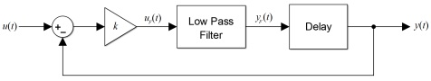
Figure 6