Reference no: EM132817900

Problem 1: Portfolio Optimization

Suppose we want to design a portfolio among following assets:

StocksArray = c(' MSFTY AAPL',' AMZN',' FB',' GOOGY GOOGLY JNJ',' JPM',' VY PG',
'T',' UNH',' MA',' HD',' INTC',' V ZY KO',' BAC',' XOM',' MRK',' DIS',' PFE',
'PEP',' CMCSA',' CV X',' ADBE',' CSCO',' NVDA',' WMT',' NFLX',' CRM',
'WFC',' MCD',' ABT',' BMY',' COST',' BA',' C',' PM',' NEE',' MDT',' ABBV',
'AMGN',' TMO',' LLY',' HON',' ACN',' IBM')

The period we consider is from 01-01-2014 to 31-12-2020. In this problem, you are allowed to use any package.

(a) Please split the data set into training set and test set with 75% data in training set and 25% data in test set.

(b) Please use training data to construct the following portfolios:
• Uniform portfolio.
• Inverted volatility portfolio
• Quintile portfolio.

Apply them on test data, draw the cumulative return and drawdown. (your budget starts from 1 dollar and assuming risk-free rate is zero.)

(c) Estimation of mean vector and covariance matrix is a critical problem in portfolio optimization. Let ∑^. be the sample covariance matrix. Instead of using ∑^. to construct the portfolios, here we would use

∑^. = ρ∑^. + (1 - ρ) Trace(∑^.)I_N/N

where N is the number of asset, I_N is the identity matrix of order N, and ρ is a real number between 0 and 1. Try different values of ρ in {0, 0.2, 0.4, 0.6, 0 8, 1}, construct the global minimum variance portfolio (GMVP)

minimize w^T∑w
subject to 1^Tw = 1, w ≥ 0, and compute the Sharpe ratio on test set.

(d) In this subproblem, instead of estimating E via sample covariance matrix, we assume E is one of M (known) covariance matrices ∑^(k) ∈ Sⁿ₊₊, k =1,... , M, in which M = 10 and ∑(k) is computed as

∑(k) = k-1/M-1∑ + M-k Trace(∑) I_N/N

where ∑ is the sample covariance matrix, N is the number of asset, and I_N is the identity matrix of order N.

We will choose the portfolio weights in order to maximize the expected return, adjusted by the worst-case risk

minimize  -μ^Tw + λ max_k=1,...,M (w^T∑^(k)w)
subject to 1^Tw = 1.

Use CVX to solve it, apply the portfolio on test set, then show the Sharpe ratio, annualized return and average drawdown for different λ ∈ {0, 1,4,10,20}.

Problem 2: Gradient Descent

Consider a linear factor model:
xt = α + βf_t + ∈_t, t = 1, 2,... T,

where x_t ∈ R^N. We estimate α and β by solving the following least-squares problem via gradient descent

minimize     ∑^T_t=1 ||Xt - α - βf_t||²
α,β

For the vector of log-returns x_t, we'll use

Stocks = c(MSFT' AAPL',' AMZN',' KB' ,GOOG')

starting from 2016-01-01 to 2019-12-31. For the factor f_t we'll use the log-return of S&P500 index in the same period. Compare the estimates you obtained to that of CVX.

Hint The objective function is a function of α∈R^N and β∈R^N

So, there are 2N variables (α₁, , α_N, , β₁,.....β_N) to optimize. Given a point (α^t, β^t), a gradient descent step updates α and β as

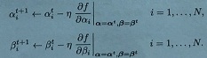
You should choose step size n and stopping criteria properly so that your algorithm converges to the optimal.

Need to use R language with CVXR package.

Attachment:- Portfolio Optimization.rar