Reference no: EM131208842

Q1. Explain carefully the difference between an unbiased estimator and a consistent estimator. Does one imply the other? If so, show mathematically, and if not provide examples.

Q2. In this question, we will use a data set on housing prices from Albuquerque, New Mexico, collected in 1993. The data set itself is called final_housingdata.dta and a description of the variables is in final_housingdata_description.txt. For the following questions, fit a linear regression with PRICE as the outcome variable, and SQFT, AGE, FEATS, NE, CUST, COR and TAX as covariates.

(a) Test whether the coefficient of FEATS is statistically significant at the 5% significance level. State the test statistic used and its null distribution.

(b) Interpret the economic (or practical) significance of SQFT on PRICE as elasticity and in terms of standard deviations.

(c) Describe the assumptions under which the test used in part (a) is valid.

(d) What expected value of housing price would you predict for a house with 3000 ft of living space, is 28 years old, has 4 features, is not located in the northeast, is a custom home, is not on the corner, and has annual taxes of $2000? Provide a point estimate and a standard error.

(e) Explain the difference between homoskedasticity and heteroskedasticity. What is the difference in terms of the assumptions of the regression model between the two cases? Give an example of why heteroskedasticity is a more reasonable assumption in this particular setting.

(f) Undr what assumptions are the OLS estimates consistent? Unbased?

Q3. Describe the omitted variable bias problem in linear regression. How does an instrumental variable addresses this problem? Explain the assumptions under which an instrumental variable is valid. What is the interpretation of the coefficient on the covariate of interest (the endogenous one) in an instrumental variable regression?

Q4. The current framework of the U.S. unemployment insurance (UI) system provides short-term monetary assistance to the involuntarily unemployed. A frequent criticism of the system has been that the unemployment insurance benefit acts as a disincentive for job-seekers and prolongs the duration of unemployment spells. During the 1980's, several controlled experiments tested alternative compensation schemes for UI. In these experiments, UI claimants were offered a cash bonus if they found a job within some specified period of time and if the job was retained for some specified duration. The question of interest was: would the promise of a monetary lump-sum benefit provide a significant inducement for more intensive job-seeking?

We consider data from the Pennsylvania reemployment bonus experiment, which was conducted in Pennsylvania from July 1988 to October 1989. The data is in f inal_pabonusdata.csv on Canvas. The variables are:

-row. names: id for person;

-duration: duration in weeks of the person's unemployment's spell;

-treatment: dummy variable for whether the person was randomly assigned to be in treatment group that is eligible to receive bonus (if treatment,=0, the person was assigned to be in the control group that just receives usual UI without any chance to receive a bonus);

-female: dummy variable for female;

-black: dummy variable for black;

-hispanic: dummy variable for Hispanic;

-ndependents: number of dependents, with 2 indicator two or more dependents;

-recall: dummy variable for whether person "expected to be recalled;"

-young: dummy variable for whether person was less than 35;

-old: dummy variable for whether person was greater than 54;

-durable: dummy variable for whether person was empoloyed in the durable goods industry;

-lusd: dummy variable for whether person lives in a low employment district (Coatesville Reading or Lancaster).               ,

We use the Weibull model. Let X_i denote the covariates for subject i and Y_i the duration of the unemployment spell for subject i.

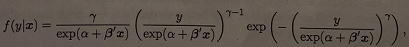
where γ > 0.

(a) Write down the log likelihood function.

(b) Use the fact that the Weibull model has the property that E(logY_i|X_i) = α + β'X_i to estimate α and β by least squares.

(c) The method of maximum likelihood is more efficient than least squares (in the normal linear regression, the maximum likelihood estimates are the same as the least squares estimates but this is not the case for the Weibull model). Estimate the parameters of the model by maximum likelihood. For one set of starting values, use the estimates in part (b) along with γ = 1. Try several other starting values. (For full credit, you will have to solve a constrained optimization problem since γ > 0. For example, to constrain γ > 0 in the optim function in R, use the options method="L-BFGS-B", lower=0, upper=Inf. See the help file for the optim function. In Matlab, you can use the fmincon function. Alternatively, you can set γ = 1.08 and get partial credit.)

(d) Find the standard errors for the maximum likelihood estimates. For which covariates would we reject the null hypothesis that the covariate has no effect on duration holding the other covariates fixed for significance level 0.05.

(e) Test whether the parameters for the old and young covariates are both equal to zero using the likelihood ratio test. (Like in part (c), you can either do a constrained optimization to get full credit, or set 7 = 1.08 and you will get partial credit.)

(f) The hazard rate at a duration y is the instantaneous rate of a duration ending given that it has lasted up until time y. For the Weibull model, the hazard rate is

h(y|x) = (γ/exp(α+β'x))(y/exp(α + β'x))^γ-1

Show that for the Weibull model, if covariate j is increased by one unit, the hazard rate for each y is multiplied by exp (β_jγ). (The fact that the hazard rate for each y is multiplied by the same factor is called the proportional hazards property.)

(g) Use the bootstrap to find an approximate 95% confidence interval for how much treatment multiplies the hazard rate compared to control when the other covariates are held fixed. (Again, you can set γ = 1.08 to get partial credit.)

(h) What do you conclude about the effect of the UI bonus treatment from the analyses you have done in (a)-(g)?

Q5. Suppose that X has the following density

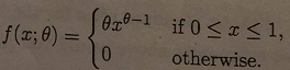
The table below shows data on a random sample X₁, ..., X₂₀ from this distribution and some summary statistics.

i	X	ln(X)
1	0.68	-0.39
2	0.16	-1.83
3	0.11	-2.25
4	0.26	-1.34
5	0.63	-0.47
6	0.59	-2.53
7	0.95	-0.05
8	0.88	-0.13
9	0.90	-0.10
10	0.86	-.015
11	0.64	-0.44
12	0.95	-0.05
13	0.27	-1.30
14	0.68	-0.39
15	0.77	-0.26
16	0.31	-1.17
17	0.79	-0.24
18	0.57	-0.57
19	0.99	-0.01
20	0.74	-0.29
Sum	12.73	-11.98
Average	0.64	-0.60

(a) Show that E(X) = (θ/1+θ). Write down the moment condition based on this equation and find an estimator for 8 using the (generalized) method of moments. Compute the estimate with the given sample.

(b) For a given θ, the random variable U^1/θ where U _~ Uniform (0, 1), has the same distribution as the random variable X (this is true and you do not need to prove it). Using this procedure to generate random draws from X, compute a 95% confidence interval using bootstrapping for the method of moments estimator derived in part (a).

(c) Find the maximum likelihood estimator (MLE) of θ (verify that your estimator is indeed the maximizer of the likelihood). Calculate the estimate with the given sample.

(d) Calculate the asymptotic standard error for the MLE estimator derived in part (c).

(e) Which of the two estimators above would you prefer and explain why.

Q6. For this question you have to use the data in the ascii file yogurt_2008.txt. The data consists of observations on 437 households making 2582 yogurt purchases. They purchase one of three brands. The five variables in the data set are, (i) the household id, running from 1 to 437, (ii) the choice, running from 1 to 3, (iii) the price, in Cents, of the yogurt brand 1, (iv) the price, in cents, of the yogurt brand 2, (v) the price, in cents, of the yogurt brand 3. Let j index the choice, running from 1 to 3, t index the purchase, running from 1 to Ti, and i the household, running from 1 to 437. The number of purchases made by each household differs. For example, the first two purchases come from household 1, the next two from household 2, and the next eight from the third household.

We focus on a discrete choice model where the utility for individual i associated with choice j, in purchase t is

U_ijt = α_j + β· P_ijt + ε_ijt,

where P_ijt is the price of brand j for household i at purchase time t. We assume the ε_ijt are independent across time, choice and household. Normalize α₁ = 0, so that there are three free parameters, α₂, α₃, and β.

(a) Calculate the mean price for each brand, by the choice made. That is, calculate the average price of brand 1, 2 and 3 for households choosing brand 1, calculate the average price of brand 1, 2 and 3 for households choosing brand 2, and calculate the average price of brand 1, 2 and 3 for households choosing brand 3. Do the patterns make sense? That is, are the prices for brand j lowest among the households choosing brand j?

(b) Suppose we want to estimate the conditional logit model. Because of the independence assumption on the E_ijt, we can ignore the fact that some purchases come from the same household, and the likelihood function is

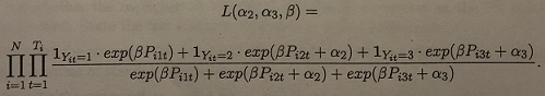
Find the maximum likelihood estimator (α^{^}2, α^{^}₃, β).

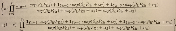
(c) Next we explore a random coefficient version of the conditional logit model. Rather than continuous mixtures, we use a simple version with a binary mixture. We will let the coefficient on price vary by household. Thus, we model the latent utility as

U_ijt = α_j + βi · P_ijt + ε_ijt,

where β_i ∈ {β_L, β_H} with Pr = (β_i = β_L) = π. Show that the likelihood function for this mixture model is

L(α2, α3, βL, βH, π) = _i=1∏^N                          

(d) Plot the log likelihood function, for π = 0.5, at

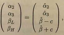
as a function of c, from c = 0 to c = 0.2. Compare the value of the log likelihood function at the value of c that maximizes it with the value at c = 0. Does it appear that allowing for the heterogeneity in price sensitivity is important?

(e) Explain why the random coefficient model might be preferred to the conditional logit model. Which (undesirable) property of the conditional logit model can we avoid by using the random coefficient model? Why is this property undesirable?