Reference no: EM132583667

Questions -

Q1. A group of senior citizens who have never used the internet before are given training over a period of 6 months. A sample of 3 of them is chosen at random and their numbers of hours of internet use are recorded for the 6 months, as shown in Figure 1.

(i) Describe briefly the data, discussing any interesting features. Based on Figure 1 only suggest the form of a possible linear model of the hours of use per month (as response variable) and month (as explanatory variable).

(ii) Let y be the hours of use per month and x be the month. An analysis in R gave the following output: (see attached file)

(a) Write down the fitted model.

(b) Comment on the model and the quality of its goodness of fit, making appropriate reference to any goodness of fit diagnostics. State clearly any hypothesis you may use.

(c) Using one of the following R extracts

> qnorm(0.95)  > qt(0.95, df=14)

[1] 1.644854  [1] 1.76131

> qt(0.95, df=15)  > qt(0.995, df=15)

[1] 1.75305  [1] 2.946713

calculate 90% confidence intervals for the coefficient of x and for the coefficient of x².

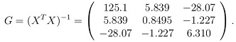
(d) For month x = 1 calculate a 90% predictive interval for the future observation y. You may use the following:

where X is the design matrix of the linear model.

(e) A further R analysis gave. Calculate the correlation coefficient of the estimator of the gradient (coefficient of x) and the estimator of the coefficient of x².

Q2. A data-set on black cherry trees in the Allegheny National Forest, Pennsylvania, USA includes the height, radius (measured 4.5 feet above the ground) and volume, for each of 31 trees.

(i) A model v_i = β₀ + β₁r_i + β₂h_i + ∈_i (1)

has been proposed, where h_i, r_i, v_i are the natural logarithms of the height (in feet), radius (in feet) and volume (in cubic feet) of the ith tree, and ∈_i ~ 1 N(0, σ²) independently for different trees. The following output summarizes the results of fitting this model in R.

Explain the hypothesis being tested by each of the three F statistics included in the output. What interpretation, if any, can be placed on their conclusions here?

(ii) Figure 2 shows the standardized deletion residuals for the model above. The following calculations can be used as the basis of a test on the standardized deletion residuals, using the Sidak correction. >alpha=0.05

> prob=1-(1-alpha)-(1/31)

> qt(prob/2,27)

[1] -3.495321

Explain the interpretation of the values alpha and prob used in the calculation, and carry out the test.

(iii) Thinking about the trunk of each tree as a cylinder, a simple geometric calculation suggests that

Vi ≈ kR_i²H_i (2)

where V_i = exp(v_i) etc., and that k ≈ π (the usual circular constant). Explain why the model suggested by (2) can be represented as a special case of (1) under the null hypothesis that β₁ = 2 and β₂ = 1, and explain how that null hypothesis can be written in the general form

Cβ = c.

Express the weaker hypothesis that β₁ + β₂ = 3 in a similar form, and calculate the corresponding F statistic, using the fact that

What is the null distribution of this F statistic?

Q3. (i) A laboratory experiment is intended to investigate the effect of a drug on certain species of micro-organisms. Tissue cultures containing set amounts of one of three species of micro-organisms (A, B, C) are each exposed to doses of the drug being tested; there are four different doses used, and two replicates of each combination of species and dose. Figure 3 shows a plot produced in R of the dose and response for each run, the points being coded by species.

Various models are being considered for the response as a function of species and dose. The output below shows summaries of results for two models; Response and Species have the obvious meaning, NumDose refers to the dose as a quantitative variable, and FacDose refers to the dose as a factor variable.

(a) Give the equations for these two models, explaining your notation and assumptions.

(b) Calculate the BIC for each of these two models. Based on the BIC, explain which of the two models you would prefer and why.

(c) What advantages and disadvantages do these two modelling approaches-dose as a factor, and dose as a numerical variable-have for this experiment, beyond those taken into account in the BIC?

(ii) Consider the linear model

y_i = x_i^Tβ + ∈_i,  i = 1, 2, . . . , n, (3)

where ∈_i is an i.i.d. sequence of random variables with zero mean and variance Var(∈_i) = σ²c_i, for some variance σ² and c_i > 0.

Discounted least squares considers the maximum likelihood estimator β^{^} of β, which minimises the discounted sum of squares

S_δ(β) = _i=1∑ⁿδ^n-i(y_i - x_i^Tβ)²,

for some discount factor δ that satisfies 0 < δ ≤ 1.

(a) Show that discounted least squares is a special case of weighted least squares (WLS) and calculate the weights of WLS as functions of δ.

(b) Using the relationship of discounted least squares and WLS as in (a), derive the variance of ∈_i as a function of σ² and δ.

(c) For the simple linear regression model with no intercept and a near constant covariate x_i ≈ x, i.e.

y_i ≈ xβ + ∈_i,  

show that

β^ = ((1- δ)/x(1- δⁿ))_i=1∑ⁿδ^n-1y_i.

Attachment:- Statistics Assignment File.rar