Reference no: EM131051263
Question 1:
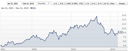
Visit the Australian Stock Exchange website, www.asx.com.au and from "Prices and research" drop-down menu, select "Company information". Type in the ASX code "CCL" (Coca-Cola Amatil Limited), and find out details about the company. Your task will be to get the opening prices of a CCL share for every quarter from January 2001 to December 2015. If you are working with the monthly prices, read the values in the beginning of every Quarter (January, April, July, October) for every year from 2001 to 2015. It is part of the assignment task to test your ability to find the information from an appropriate website. If you are unable to do so, you may read the values from the chart provided below obtained from Etrade Australia. Obviously, reading from the chart will not be accurate and you may expect around 60 percent marks with such inaccuracy. After you have recorded the share prices, answer the following questions:
(a) List all the values in a table and then construct a stem-and-leaf display for the data.
(b) Construct a relative frequency histogram for these data with equal class widths, the first class being "$4 to less than $6".
(c) Briefly describe what the histogram and the stem-and-leaf display tell you about the data. What effects would there be if the class width is doubled, which means the first class will be "$4 to less than $8"?
(d) What proportion of stock prices were above $10?
(Note: Use only the original values of share prices and not adjusted values.)
Question 2:
The following table provides the median weekly rents of a 3-bedroom house of a few randomly selected suburbs in four capital cities of Australia - Sydney, Melbourne, Brisbane and Perth - for March 2016. The data is obtained from the website https://www.realestate.com.au/neighbourhoods/. From the data answer the questions below for the capital cities.
Median weekly rent of a 3 bedroom house In Australian capital cities
| Sydney |
Melbourne |
Brisbane |
Perth |
| Suburb name |
Rent ($) |
Suburb name |
Rent ($) |
Suburb name |
Rent ($) |
Suburb name |
Rent ($) |
| Newtown |
890 |
Carkon |
700 |
Fortitude Valey |
610 |
Stbaco |
725 |
| Ranchvick |
999 |
Footsaay |
413 |
Wookoongabba |
480 |
Innaloo |
470 |
| Maroubra |
850 |
Kew |
645 |
McDowell |
450 |
Balculta |
395 |
| Rockdale |
600 |
Toorak |
895 |
Underwood |
395 |
Duncrarg |
440 |
| Camsie |
550 |
Coburg |
480 |
Manly |
450 |
Dalkeirn |
715 |
| Hurstwile |
580 |
Camberwell |
605 |
Jindalee |
415 |
Bassendean |
400 |
| Auburn |
485 |
Ringwood |
380 |
Cleveland |
425 |
Kewdale |
395 |
| Ryde |
650 |
Moorabbin |
465 |
Teneriffe |
700 |
Beckenham |
380 |
| Cabramatta |
420 |
Wernbee |
300 |
Tingalpa |
420 |
Langford |
340 |
| Bella Vista |
658 |
Truganna |
330 |
Algester |
390 |
Kardinya |
430 |
| Artarmon |
950 |
Taylors Lakes |
370 |
Aspley |
420 |
Cottesloe |
800 |
| Bankstown |
500 |
Bundoora |
370 |
Herston |
535 |
Stratton |
350 |
| Chatswood |
850 |
Craigiebum |
340 |
New Farm |
685 |
|
|
| Epping |
630 |
Epping |
340 |
|
|
|
|
|
|
Pod Melbourne |
813 |
|
|
|
|
(a) Compute the mean, median, first quartile, and third quartile for each capital city (with only the data provided for that city, do not add/delete values for any new/given suburb of question 2) using the exact position, (n+1)f, where n is the number of observations and f the relevant fraction for the quartile.
(b) Compute the standard deviation, range and coefficient of variation from the sample data for each city.
(c) Draw a box and whisker plot for the median weekly rents of each city and put them side by side on the same scale so that the prices can be compared.
(d) Compare the box plots and comment on the distribution of the data.
Question 3:
The Table below is taken from the Australian Bureau of Statistics website. It provides data on energy use of households - almost all houses use mains electricity but some use additional energy sources such as gas and solar. (You can get the data from Table 1 from the URL: https://www.abs.gov.au/AUSSTATS/[email protected]/DetailsPage/4602.0.55.001Mar%202014?OpenDocument.) Missing cells indicate data not published, and totals may be higher since all possibilities may not be listed. The totals are not incorrect.).
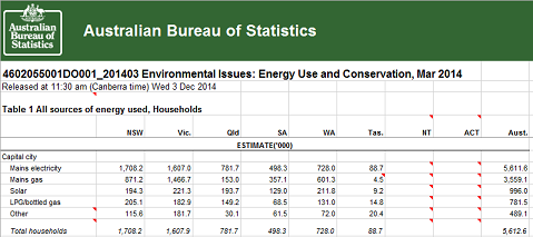
Based on the information available in the table above -
(a) What is the probability that an Australian household, randomly selected, uses solar as a source of energy?
(b) What is the probability that an Australian household, randomly selected, uses mains gas and is located in Victoria?
(c) Given that a household uses LPG/bottled gas, what is the probability that the household is located in South Australia?
(d) Is the percentage of Australian households using mains gas independent of the state?
Question 4:
(a) The following data collected from the Australian Bureau of Meteorology Website (https://www.bom.gov.au/climate/data/?ref=ftr) gives the daily rainfall data for the year 2015 in Brisbane. The zero values indicate no rainfall and the left-most column gives the date. Assuming that the weekly rainfall event (number of days in a week with rainfall) follows a Poisson distribution (There are 52 weeks in a year and a week is assumed to start from Monday. The first week starts from 29 December 2014 - you are expected to visit the website and get the daily values which are not given in the table below. Make sure you put the correct station number. Ignore the last few days of 2015 if it exceeds 52 weeks.):
(i) What is the probability that on any given week in a year there would be no rainfall?
(ii) What is the probability that there will be 2 or more days of rainfall in a week?
Observations of Dail) rainfall are nominally made at 9 am local clock time and record the total for the preaous 24 hours. Rainfall includes all forms of precipitation that reach the ground, such as rain, drizzle, had and snow. About rainfall data
Station: Brisban Number 40913 Opened: 1999 Now: Open
Lat 27.48's Lon:153.04*E Elevation: 8m
Key: Units = mm 12.3= Not Quality controlled = Pan of accumulated total
| 2015 |
Jan |
Feb |
Mar |
Apr |
May |
Jun |
Jul |
Aug |
Sep |
Oct |
Nov |
Dec |
| Graph |
|
|
|
|
|
|
|
|
|
|
|
|
| 1st |
12.2 |
17.2 |
0 |
68.2 |
56.2 |
0 |
0.2 |
0 |
0 |
0 |
0 |
0 |
| 2nd |
0.2 |
0 |
0 |
8.8 |
182.6 |
0 |
0 |
0 |
|
0 |
0 |
0.4 |
| 3rd |
1.2 |
2.2 |
0 |
38.4 |
0 |
0 |
0 |
0 |
2.4 |
0 |
0 |
2 |
| 4th |
16.8 |
0 |
0 |
0.4 |
0 |
0 |
0 |
0 |
0.2 |
0 |
11.6 |
0.2 |
| 5th |
0 |
0 |
0 |
1.8 |
0 |
0 |
0 |
0 |
0 |
0 |
0 |
0 |
| 6th |
21.6 |
2.8 |
0 |
0 |
|
0 |
0 |
0 |
0 |
0 |
19 |
0 |
| 7th |
0 |
0.2 |
0 |
0 |
0 |
0 |
0 |
0 |
0 |
0 |
0 |
0 |
| 8th |
1.8 |
0.2 |
0 |
0 |
|
0.2 |
0 |
0 |
0 |
0 |
0.4 |
0 |
| 9th |
3.6 |
0 |
0 |
0 |
0 |
0 |
0 |
0 |
0 |
5.8 |
14 |
0 |
| 10th |
0 |
5.2 |
0 |
0 |
0 |
0 |
2 |
0 |
0 |
0.2 |
0 |
0 |
| 11th |
0 |
12.2 |
0 |
0 |
0 |
0 |
0 |
0 |
0 |
0 |
0 |
0.6 |
| 12th |
14.6 |
8.4 |
0 |
0 |
0 |
4.6 |
0.6 |
0.2 |
0 |
0 |
0 |
1 |
| 13th |
38.6 |
1.6 |
0 |
0 |
0 |
1.2 |
0.2 |
3.6 |
0 |
0 |
0 |
9.8 |
| 14th |
0.2 |
0.4 |
0 |
0 |
0 |
4.2 |
0 |
0 |
0 |
0.2 |
1 |
0.8 |
| 15th |
|
0.2 |
0 |
0 |
0 |
4 |
0 |
0 |
0 |
4.4 |
10.6 |
0 |
| 16th |
0 |
0.4 |
0 |
0.2 |
0 |
1 |
0 |
0 |
0 |
0 |
0.2 |
0 |
| 17th |
0 |
0.4 |
0 |
0 |
1 |
3.4 |
0 |
0 |
10.2 |
0 |
0.6 |
3.8 |
| 18th |
0 |
0.2 |
0 |
3.4 |
6.6 |
2.4 |
0 |
0 |
18 |
0 |
0 |
3.2 |
| 19th |
0 |
4.6 |
7.6 |
0.4 |
0.8 |
0 |
0 |
0 |
0.6 |
0 |
0 |
0 |
| 20th |
35.8 |
54 |
0 |
14.6 |
0 |
0 |
0 |
0 |
0 |
0 |
0 |
0 |
| 21st |
0.2 |
89.2 |
0.2 |
2 |
0.2 |
0 |
0.2 |
0.4 |
1.6 |
0 |
0 |
0 |
| 22nd |
1 |
68.4 |
68 |
0.2 |
1.4 |
0 |
2.8 |
2.2 |
0 |
0 |
0 |
0 |
| 23rd |
100.4 |
4.4 |
81.8 |
0 |
0 |
0 |
4.4 |
0 |
0 |
20.8 |
0 |
0 |
| 24th |
65.2 |
0.4 |
0 |
0 |
0 |
0 |
0 |
0 |
0.6 |
0 |
0 |
3.2 |
| 25th |
0 |
0.2 |
0 |
0 |
0 |
0 |
0 |
2.2 |
0.2 |
1.2 |
0 |
9.2 |
| 26th |
0 |
1.8 |
3.8 |
0 |
0 |
0.2 |
0.2 |
0 |
0 |
0 |
0 |
0.4 |
| 27th |
0 |
0.2 |
0 |
0 |
|
0 |
0 |
0 |
0.4 |
4.8 |
0 |
0.8 |
| 28th |
5.2 |
|
0 |
0 |
0 |
2.4 |
0 |
5 |
12.2 |
13.2 |
0 |
0.8 |
| 29th |
0 |
|
0 |
|
0 |
7 |
0 |
0.2 |
0 |
5 |
0 |
0 |
| 30th |
3.8 |
|
0 |
7.8 |
4 |
4 |
0 |
13.6 |
7.8 |
0.2 |
0.2 |
0 |
| 31st |
0 |
|
0 |
|
0 |
|
0 |
0.2 |
|
0 |
16.6 |
0 |
| Highest Daily |
100.4 |
89.2 |
81.8 |
68.2 |
182.6 |
7 |
4.4 |
13.6 |
18 |
20.8 |
19 |
9.8 |
| Monthly Total |
322.4 |
274.8 |
161.4 |
146.2 |
248.8 |
34.6 |
9.2 |
27.6 |
54.2 |
55.6 |
74.2 |
36.2 |
(b) Assuming that the weekly total amount of rainfall (in mm) from the data provided in part (a) has a normal distribution, compute the mean and standard deviation of weekly totals.
(i) What is the probability that in a given week there will be between 5 mm and 10 mm of rainfall?
(ii) What is the amount of rainfall if only 13% of the weeks have that amount of rainfall or higher?
Question 5:
The following data is taken from the UCI machine learning data repository (https://archive.ics.uci.edu/ml/datasets/Wine+Quality). It lists a few attributes of red wine, randomly sampled from thousands of bottles, which can be classified as of good, medium and poor quality.
(a) Test for normality of all the variables separately for good wine using normal probability plot.
(b) Construct a 95% confidence interval for each of the variables for good wine.
(c) Find the mean of each of the variables for medium quality red wine. Do the same for the poor quality red wine.
(d) Check if the means calculated for the medium and poor quality red wines fall within the corresponding confidence intervals of the good quality wine. For those attributes whose means lie outside the confidence interval, the attributes are significant in determining the quality. This assumption is, however, partially compromised if the attribute fails the normality test. Identify the significant and non-significant variables, and comment.
|
Good quality red wine
|
|
Alcohol
|
Residual sugar
|
Chlorides
|
Total sulfur dioxide
|
Density
|
pH
|
Sulphates
|
Citric acid
|
|
10
|
1.2
|
0.065
|
21
|
0.9946
|
3.39
|
0.47
|
0
|
|
9.5
|
2
|
0.073
|
18
|
0.9968
|
3.36
|
0.57
|
0.02
|
|
10.5
|
1.8
|
0.092
|
103
|
0.9969
|
3.3
|
0.75
|
0.56
|
|
9.7
|
2.1
|
0.066
|
30
|
0.9968
|
3.23
|
0.73
|
0.28
|
|
9.5
|
1.9
|
0.085
|
35
|
0.9968
|
3.38
|
0.62
|
0.16
|
|
10.5
|
1.8
|
0.065
|
16
|
0.9962
|
3.42
|
0.92
|
0.16
|
|
13
|
1.2
|
0.046
|
93
|
0.9924
|
3.57
|
0.85
|
0.08
|
|
10.3
|
1.4
|
0.056
|
24
|
0.99695
|
3.22
|
0.82
|
0.47
|
|
10.8
|
2.6
|
0.095
|
28
|
0.9994
|
3.2
|
0.77
|
0.74
|
|
10.8
|
2.6
|
0.095
|
28
|
0.9994
|
3.2
|
0.77
|
0.74
|
|
10.5
|
2.1
|
0.054
|
19
|
0.998
|
3.31
|
0.88
|
0.58
|
|
12.2
|
1.6
|
0.054
|
106
|
0.9927
|
3.54
|
0.62
|
0.04
|
|
9.2
|
2.2
|
0.075
|
24
|
1.00005
|
3.07
|
0.84
|
0.44
|
|
9.2
|
2.2
|
0.075
|
24
|
1.00005
|
3.07
|
0.84
|
0.44
|
|
10.5
|
2.6
|
0.085
|
33
|
0.99965
|
3.36
|
0.8
|
0.47
|
|
10.2
|
1.8
|
0.071
|
10
|
0.9968
|
3.2
|
0.72
|
0.52
|
|
12.8
|
3.6
|
0.078
|
37
|
0.9973
|
3.35
|
0.86
|
0.46
|
|
12.6
|
6.4
|
0.073
|
13
|
0.9976
|
3.23
|
0.82
|
0.45
|
|
10.5
|
5.6
|
0.087
|
47
|
0.9991
|
3.38
|
0.77
|
0.32
|
|
9.9
|
3.5
|
0.358
|
10
|
0.9972
|
3.25
|
1.08
|
0.68
|
|
10.5
|
5.6
|
0.087
|
47
|
0.9991
|
3.38
|
0.77
|
0.32
|
|
10.6
|
2.5
|
0.091
|
49
|
0.9976
|
3.34
|
0.86
|
0.09
|
|
10.6
|
2.5
|
0.091
|
49
|
0.9976
|
3.34
|
0.86
|
0.09
|
|
11.5
|
3.2
|
0.083
|
59
|
0.9989
|
3.37
|
0.71
|
0.39
|
|
11.5
|
3.2
|
0.083
|
59
|
0.9989
|
3.37
|
0.71
|
0.39
|
|
11.5
|
3.65
|
0.121
|
14
|
0.9978
|
3.05
|
0.74
|
0.66
|
|
11.7
|
2.5
|
0.078
|
38
|
0.9963
|
3.34
|
0.74
|
0.01
|
|
12.2
|
3.4
|
0.128
|
21
|
0.9992
|
3.17
|
0.84
|
0.53
|
|
9.8
|
2.3
|
0.082
|
29
|
0.9997
|
3.11
|
1.36
|
0.54
|
|
12.3
|
2.7
|
0.072
|
34
|
0.9955
|
3.58
|
0.89
|
0.02
|
|
11.7
|
2.95
|
0.116
|
29
|
0.997
|
3.24
|
0.75
|
0.66
|
|
10.4
|
3.1
|
0.109
|
23
|
1
|
3.15
|
0.85
|
0.66
|
|
10
|
5.8
|
0.083
|
42
|
1.0022
|
3.07
|
0.73
|
0.66
|
|
10
|
5.8
|
0.083
|
42
|
1.0022
|
3.07
|
0.73
|
0.66
|
|
12
|
2.4
|
0.074
|
18
|
0.9962
|
3.2
|
1.13
|
0.53
|
|
11.8
|
4.4
|
0.124
|
15
|
0.9984
|
3.01
|
0.83
|
0.71
|
|
12
|
2.4
|
0.074
|
18
|
0.9962
|
3.2
|
1.13
|
0.53
|
|
10
|
2.5
|
0.096
|
49
|
0.9982
|
3.19
|
0.7
|
0.31
|
|
12.9
|
1.4
|
0.045
|
88
|
0.9924
|
3.56
|
0.82
|
0.05
|
|
13
|
4.2
|
0.066
|
38
|
1.0004
|
3.22
|
0.6
|
0.76
|
|
10.8
|
3
|
0.093
|
30
|
0.9996
|
3.18
|
0.63
|
0.66
|
|
11.7
|
6.7
|
0.097
|
19
|
0.9986
|
3.27
|
0.82
|
0.53
|
|
11.8
|
2.4
|
0.089
|
67
|
0.9972
|
3.28
|
0.73
|
0.33
|
|
12.3
|
2.3
|
0.059
|
48
|
0.9952
|
3.52
|
0.56
|
0.03
|
|
11
|
2.1
|
0.066
|
24
|
0.9978
|
3.15
|
0.9
|
0.47
|
|
12.3
|
2.3
|
0.059
|
48
|
0.9952
|
3.52
|
0.56
|
0.03
|
|
11
|
2.1
|
0.066
|
24
|
0.9978
|
3.15
|
0.9
|
0.47
|
|
9.8
|
2.2
|
0.072
|
29
|
0.9987
|
2.88
|
0.82
|
0.72
|
|
11.2
|
3.7
|
0.1
|
43
|
1.0032
|
2.95
|
0.68
|
0.76
|
|
11.6
|
2.7
|
0.077
|
19
|
0.9963
|
3.23
|
0.63
|
0.49
|
|
12.5
|
1.7
|
0.054
|
27
|
0.9934
|
3.57
|
0.84
|
0.01
|
|
11.2
|
2.8
|
0.084
|
22
|
0.9998
|
3.26
|
0.74
|
0.63
|
|
13.4
|
5.2
|
0.086
|
19
|
0.9988
|
3.22
|
0.69
|
0.67
|
|
11.2
|
2.8
|
0.084
|
22
|
0.9998
|
3.26
|
0.74
|
0.63
|
|
11.7
|
2.8
|
0.08
|
17
|
0.9964
|
3.15
|
0.92
|
0.56
|
|
10.8
|
2.8
|
0.081
|
67
|
1.0002
|
3.32
|
0.92
|
0.55
|
|
13.3
|
2.5
|
0.055
|
25
|
0.9952
|
3.34
|
0.79
|
0.5
|
|
13.4
|
2.6
|
0.052
|
27
|
0.995
|
3.32
|
0.9
|
0.51
|
|
11
|
2.6
|
0.07
|
16
|
0.9972
|
3.15
|
0.65
|
0.53
|
|
11
|
2.6
|
0.07
|
16
|
0.9972
|
3.15
|
0.65
|
0.53
|
|
12
|
6.55
|
0.074
|
76
|
0.999
|
3.17
|
0.85
|
0.73
|
|
12
|
6.55
|
0.074
|
76
|
0.999
|
3.17
|
0.85
|
0.73
|
|
10.9
|
1.9
|
0.078
|
24
|
0.9976
|
3.18
|
1.04
|
0.47
|
|
10.8
|
1.8
|
0.077
|
22
|
0.9976
|
3.21
|
1.05
|
0.42
|
|
12.5
|
2.9
|
0.072
|
26
|
0.9968
|
3.16
|
0.78
|
0.63
|
|
10.8
|
1.8
|
0.075
|
21
|
0.9976
|
3.25
|
1.02
|
0.46
|
|
11.4
|
2.8
|
0.084
|
43
|
0.9986
|
3.04
|
0.68
|
0.75
|
|
11.8
|
2.4
|
0.107
|
15
|
0.9973
|
3.09
|
0.66
|
0.64
|
|
11.8
|
2.4
|
0.107
|
15
|
0.9973
|
3.09
|
0.66
|
0.64
|
|
Medium quality red wine
|
|
alcohol
|
residual sugar
|
chlorides
|
total sulfur dioxide
|
density
|
pH
|
sulphates
|
citric acid
|
|
9.4
|
1.9
|
0.076
|
34
|
0.9978
|
3.51
|
0.56
|
0
|
|
9.8
|
2.6
|
0.098
|
67
|
0.9968
|
3.2
|
0.68
|
0
|
|
9.8
|
2.3
|
0.092
|
54
|
0.997
|
3.26
|
0.65
|
0.04
|
|
9.4
|
1.9
|
0.076
|
34
|
0.9978
|
3.51
|
0.56
|
0
|
|
9.4
|
1.8
|
0.075
|
40
|
0.9978
|
3.51
|
0.56
|
0
|
|
9.4
|
1.6
|
0.069
|
59
|
0.9964
|
3.3
|
0.46
|
0.06
|
|
10.5
|
6.1
|
0.071
|
102
|
0.9978
|
3.35
|
0.8
|
0.36
|
|
9.2
|
1.8
|
0.097
|
65
|
0.9959
|
3.28
|
0.54
|
0.08
|
|
10.5
|
6.1
|
0.071
|
102
|
0.9978
|
3.35
|
0.8
|
0.36
|
|
9.9
|
1.6
|
0.089
|
59
|
0.9943
|
3.58
|
0.52
|
0
|
|
9.1
|
1.6
|
0.114
|
29
|
0.9974
|
3.26
|
1.56
|
0.29
|
|
9.2
|
3.8
|
0.176
|
145
|
0.9986
|
3.16
|
0.88
|
0.18
|
|
9.2
|
3.9
|
0.17
|
148
|
0.9986
|
3.17
|
0.93
|
0.19
|
|
9.3
|
1.7
|
0.368
|
56
|
0.9968
|
3.11
|
1.28
|
0.28
|
|
9.7
|
2.3
|
0.082
|
71
|
0.9982
|
3.52
|
0.65
|
0.31
|
|
9.5
|
1.6
|
0.106
|
37
|
0.9966
|
3.17
|
0.91
|
0.21
|
|
9.4
|
2.3
|
0.084
|
67
|
0.9968
|
3.17
|
0.53
|
0.11
|
|
9.3
|
1.4
|
0.08
|
23
|
0.9955
|
3.34
|
0.56
|
0.16
|
|
9.5
|
1.8
|
0.08
|
11
|
0.9962
|
3.28
|
0.59
|
0.24
|
|
9.5
|
1.6
|
0.106
|
37
|
0.9966
|
3.17
|
0.91
|
0.21
|
|
9.4
|
1.9
|
0.08
|
35
|
0.9972
|
3.47
|
0.55
|
0
|
|
10.1
|
2.4
|
0.089
|
82
|
0.9958
|
3.35
|
0.54
|
0.07
|
|
9.8
|
2.3
|
0.083
|
113
|
0.9966
|
3.17
|
0.66
|
0.12
|
|
9.2
|
1.8
|
0.103
|
50
|
0.9957
|
3.38
|
0.55
|
0.25
|
|
10.5
|
5.9
|
0.074
|
87
|
0.9978
|
3.33
|
0.83
|
0.36
|
|
10.5
|
5.9
|
0.074
|
87
|
0.9978
|
3.33
|
0.83
|
0.36
|
|
10.3
|
2.2
|
0.069
|
23
|
0.9968
|
3.3
|
1.2
|
0.22
|
|
9.5
|
1.8
|
0.05
|
11
|
0.9962
|
3.48
|
0.52
|
0.02
|
|
9.2
|
2.2
|
0.114
|
114
|
0.997
|
3.25
|
0.73
|
0.43
|
|
9.5
|
1.6
|
0.113
|
37
|
0.9969
|
3.25
|
0.58
|
0.52
|
|
9.2
|
1.6
|
0.066
|
12
|
0.9958
|
3.34
|
0.56
|
0.23
|
|
9.2
|
1.4
|
0.074
|
96
|
0.9954
|
3.32
|
0.58
|
0.37
|
|
9.2
|
1.7
|
0.074
|
23
|
0.9971
|
3.15
|
0.74
|
0.26
|
|
9.4
|
3
|
0.081
|
119
|
0.997
|
3.2
|
0.56
|
0.36
|
|
9.5
|
3.8
|
0.084
|
45
|
0.9978
|
3.34
|
0.53
|
0.04
|
|
9.6
|
3.4
|
0.07
|
10
|
0.9971
|
3.04
|
0.63
|
0.57
|
|
9.4
|
5.1
|
0.111
|
110
|
0.9983
|
3.26
|
0.77
|
0.12
|
|
10
|
2.3
|
0.076
|
54
|
0.9975
|
3.43
|
0.59
|
0.18
|
|
9.2
|
2.2
|
0.079
|
52
|
0.998
|
3.44
|
0.64
|
0.4
|
|
9.3
|
1.8
|
0.115
|
112
|
0.9968
|
3.21
|
0.71
|
0.49
|
|
9.8
|
2
|
0.081
|
54
|
0.9966
|
3.39
|
0.57
|
0.05
|
|
10.9
|
4.65
|
0.086
|
11
|
0.9962
|
3.41
|
0.39
|
0.05
|
|
10.9
|
4.65
|
0.086
|
11
|
0.9962
|
3.41
|
0.39
|
0.05
|
|
9.6
|
1.5
|
0.079
|
39
|
0.9968
|
3.42
|
0.58
|
0.11
|
|
10.7
|
1.6
|
0.076
|
15
|
0.9962
|
3.44
|
0.58
|
0.07
|
|
10.7
|
2
|
0.074
|
65
|
0.9969
|
3.28
|
0.79
|
0.57
|
|
9.5
|
2.1
|
0.088
|
96
|
0.9962
|
3.32
|
0.48
|
0.23
|
|
9.5
|
1.9
|
0.084
|
94
|
0.9961
|
3.31
|
0.48
|
0.22
|
|
9.6
|
2.5
|
0.094
|
83
|
0.9984
|
3.28
|
0.82
|
0.54
|
|
10.5
|
2.2
|
0.093
|
42
|
0.9986
|
3.54
|
0.66
|
0.64
|
|
10.5
|
2.2
|
0.093
|
42
|
0.9986
|
3.54
|
0.66
|
0.64
|
|
10.1
|
2
|
0.086
|
80
|
0.9958
|
3.38
|
0.52
|
0.12
|
|
9.2
|
1.6
|
0.069
|
15
|
0.9958
|
3.41
|
0.56
|
0.2
|
|
9.4
|
1.9
|
0.464
|
67
|
0.9974
|
3.13
|
1.28
|
0.7
|
|
9.1
|
2
|
0.086
|
73
|
0.997
|
3.36
|
0.57
|
0.47
|
|
9.4
|
1.8
|
0.401
|
51
|
0.9969
|
3.16
|
1.14
|
0.26
|
|
Poor quality red wine
|
|
alcohol
|
residual sugar
|
chlorides
|
total sulfur dioxide
|
density
|
pH
|
sulphates
|
citric acid
|
|
9
|
2.2
|
0.074
|
47
|
1.0008
|
3.25
|
0.57
|
0.66
|
|
8.4
|
2.1
|
0.2
|
16
|
0.9994
|
3.16
|
0.63
|
0.49
|
|
10.7
|
4.25
|
0.097
|
14
|
0.9966
|
3.63
|
0.54
|
0
|
|
9.9
|
1.5
|
0.145
|
48
|
0.99832
|
3.38
|
0.86
|
0.42
|
|
11
|
3.4
|
0.084
|
11
|
0.99892
|
3.48
|
0.49
|
0.02
|
|
10.9
|
2.1
|
0.137
|
9
|
0.99476
|
3.5
|
0.4
|
0
|
|
9.8
|
1.2
|
0.267
|
29
|
0.99471
|
3.32
|
0.51
|
0
|
|
10.2
|
5.7
|
0.082
|
14
|
0.99808
|
3.4
|
0.52
|
0.05
|
|
9.95
|
1.8
|
0.078
|
12
|
0.996
|
3.55
|
0.63
|
0.02
|
|
9
|
4.4
|
0.086
|
29
|
0.9974
|
3.38
|
0.5
|
0.08
|
|
9.8
|
1.5
|
0.172
|
19
|
0.994
|
3.5
|
0.48
|
0.09
|
|
9.3
|
2.8
|
0.088
|
46
|
0.9976
|
3.26
|
0.51
|
0.3
|
|
13.1
|
2.1
|
0.054
|
65
|
0.9934
|
3.9
|
0.56
|
0.15
|
|
9.2
|
2.1
|
0.084
|
43
|
0.9976
|
3.31
|
0.53
|
0.26
|
|
9.1
|
1.5
|
0.08
|
119
|
0.9972
|
3.16
|
1.12
|
0.2
|
|
10.5
|
1.4
|
0.045
|
85
|
0.9938
|
3.75
|
0.48
|
0.04
|
|
9.4
|
3.4
|
0.61
|
69
|
0.9996
|
2.74
|
2
|
1
|
|
9.2
|
1.3
|
0.072
|
20
|
0.9965
|
3.17
|
1.08
|
0.02
|
|
9
|
1.6
|
0.072
|
42
|
0.9956
|
3.37
|
0.48
|
0.03
|
|
9.1
|
1.8
|
0.058
|
8
|
0.9972
|
3.36
|
0.33
|
0.03
|
|
11.4
|
2.1
|
0.061
|
31
|
0.9948
|
3.51
|
0.43
|
0.06
|
|
10.4
|
2
|
0.089
|
55
|
0.99745
|
3.31
|
0.57
|
0.36
|
|
9.4
|
2
|
0.087
|
67
|
0.99565
|
3.35
|
0.6
|
0.04
|
|
9.8
|
3.3
|
0.096
|
61
|
1.00025
|
3.6
|
0.72
|
0
|
|
9.6
|
4.5
|
0.07
|
49
|
0.9981
|
3.05
|
0.57
|
0.49
|
|
9.6
|
2.1
|
0.07
|
47
|
0.9991
|
3.3
|
0.56
|
0.49
|
|
10
|
2.3
|
0.103
|
14
|
0.9978
|
3.34
|
0.52
|
0.24
|
|
10
|
2.1
|
0.088
|
23
|
0.9962
|
3.26
|
0.47
|
0.27
|
|
11.3
|
3.4
|
0.105
|
86
|
1.001
|
3.43
|
0.64
|
0.22
|
|
11
|
2.2
|
0.07
|
14
|
0.9967
|
3.32
|
0.58
|
0.01
|
|
11
|
4.4
|
0.096
|
13
|
0.997
|
3.41
|
0.57
|
0.02
|
|
9.6
|
2.6
|
0.073
|
84
|
0.9972
|
3.32
|
0.7
|
0.48
|
|
9.7
|
1.6
|
0.078
|
14
|
0.998
|
3.29
|
0.54
|
0.04
|
|
11.2
|
3.1
|
0.086
|
12
|
0.9958
|
3.54
|
0.6
|
0.1
|
|
11.4
|
2.1
|
0.102
|
7
|
0.99462
|
3.44
|
0.58
|
0.24
|
|
10.9
|
2.5
|
0.058
|
9
|
0.99632
|
3.38
|
0.55
|
0.07
|
|
9.9
|
1.6
|
0.147
|
51
|
0.99836
|
3.38
|
0.86
|
0.44
|