Reference no: EM132310939
R exercises
Use the NHES data to answer questions 1-3. The data dictionary for this data set is in the file named NHES data dictionary.
1. Take the first 50 samples of NHES data (only for this question), use the information on weight from years 1971 (wt71) and 1982 (wt82), rank these people individually for both the years, and generate a variable named ‘d' giving the difference in ranks. Now write a generic function to compute spearman's rank correlation using the formula:
???? = (1 -(6 ∑ni=1d2i)/N3-N)
where d is the difference in ranks and N is the sample size. Compute the rank correlation between wt71 and wt82 using your function.
2. Plot the distributions of diastolic blood pressure (dbp) and systolic blood pressure (sbp) by sex and death. Use only one graph to do this. I don't mind if they overlap or sit on top of each other. Label your graphs properly, show the differences using different colour schemes [ mark for correct boxplot commands, mark for the plot titles and proper labelling, mark for proper axis limits, mark for presenting the summaries of the boxplots (e.g. lower, upper, 75th 25th and median values)]
3. In a single plot, create histograms of birthplace for males and females. Use different colours to differentiate histograms of male and female birthplace; however, in the first instance, do not use transparent colours. Then create a second identical plot, but use transparency in the colours to more clearly display the histograms for males and females. You can use internet to search how to get transparency in the histogram plots. The two histogram plots for male and female must be done in one plot. The plots with and without transparency must be done in 1 plot area but as two separate plots. [ mark for first set of histograms, mark for the second set of histograms, mark for proper titles, mark for code].
4. Write an R function for Fisher's exact test and compute the probabilities associated with each of the below set of frequencies
|
Scenario
|
A
|
B
|
C
|
D
|
|
1
|
0
|
6
|
9
|
1
|
|
2
|
1
|
5
|
8
|
2
|
|
3
|
2
|
4
|
7
|
3
|
|
4
|
3
|
3
|
6
|
4
|
|
5
|
4
|
2
|
5
|
5
|
|
6
|
5
|
1
|
4
|
6
|
|
7
|
6
|
0
|
3
|
7
|
Do the computation using a loop and without a loop. Show both programs. Present your results in a nice table, round the probabilities to 3 digits. Fishers exact test formula is given by
[((?? + ??)! (?? + ??)! (?? + ??)! (?? + ??)!)/??! ??! ??! ??! ??!]
??h?????? ?? = (?? + ?? + ?? + ??) and ! is to be read as factorial. [ mark for function without loop, mark for function with loop, mark for showing how you rounded the final table, mark for presentation]
5. Write a generic function to generate the following sequence; 1 4 3 6 5 8 7 10 9 12, for the first n=100 numbers. Show your output till it matches this sequence. Use smart logic. Also do state if you enjoyed writing this program. [ mark for code, mark for presentation and mark for smart logic and mark for enjoyment]
STATA Exercise
We will use two different data sets 1) NHES data and 2) Socatt data. Details of Socatt data can be found in the document titled socatt.docx.
6. Read the NHES.csv into Stata and save it as a dta file. In the NHES data, there are three columns: year of death (yrdth), month of death (modth) and day of death (dadth).Combine these three columns into one column with proper format of date in yy/mm/dd. Show your
code used to convert this data, and also show your output for the first 10 rows of your data with all the three original columns (yrdth, modth, dadth) and the newly formed column. [mark for saving the data as dta file, mark for the code and for the output; show code
for saving file]
7. Using a loop and macros, compute and display summaries of the following variables for male and female: blood pressure systolic (sbp), blood pressure diastolic (dbp), weight 71 (wt71), weight 82 (wt82), height (ht), income, race, marital status, education, and age (age).
Additionally, convert your code into a basic program (an .ado file) that can be used to compute summary statistics for a given input variable and save results into a separate file. [marks for code and marks for presentation]
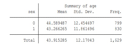
8. Using the sex and age variables from the NHES data, try to produce the below output. Use only a single line of code. Use either stata help or Google.
9. Read the Scoatt.csv file into Stata and save it as a Stata data file, then reshape the Scoatt data into wide format. Choose your variables to appropriately reshape the data. Using the data dictionary provided, code the variable names and value labels to your data. Show your code and display the top ten lines of your reshaped data set; please do not worry if all the variables do not appear in the output, select only few columns of output to fit a page. This output must show all the variable and value labels. [mark for reshape, mark for output, mark for properly labelling your variables using the code book provided and mark for presentation]
10. Using Scoatt data, do a boxplot of age by gender for each district (select only districts 35-41). This is a single panel plot area with multiple boxplots within it. See that the color of each boxplot is different. [mark for code with the command for colour, mark for placing legends and titles and 1 mark for presentation]
11. Use the long form Scoatt data to do this exercise. Write the code to select the first observation of each respondent. Show your code, and present the top ten lines of your new subset data.
Using the subset data, present your summary statistics as if it is ready to be published for the following variables: number of positive responses, party chosen, self-assessed social class, gender, and religion. Compute the summaries for the variable age in years, where the
frequencies of district is >= 8. [ mark for sub-setting data, mark for presentation of summaries, mark for age summaries and for the code defining value labels]
Attachment:- Statistical Data.rar