Reference no: EM133904015

Control

QUESTION 1

Consider the following system:

T(s) = Y(s)/U(s) = 18(s+0.2)/(s+3)(s+7)

a. Derive state space model matrices in the controller canonical form.

b. Create a new Simulink model to show that the step responses of the two representations (linear state-space system and Laplace-domain transfer function) are identical. Set the simulation time to 5.

c. If state-variable feedback control is applied, using pole-placement methodology, determine the coefficients of the state feedback gain matrix such that the closed- loop poles have values -23 and -9.

Using the characteristic polynomial of the new system, determine the eigenvalues, and hence pole position. Show that the eigenvalues are the position values of the new poles.

Create a new Simulink model to compare a modified State-Space model that includes the new state feedback gain matrix. Compare the output of this model with the output from an equivalent system in transfer function representation. Set the simulation time to 3.

QUESTION 2

A robot force control system with unity feedback shown in Figure 1 has a loop transfer function:

L(s) KG(s) = K(s+8)(s+4)(s-12)(s-3)

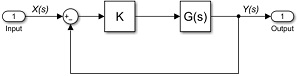
Figure 1 Unity feedback system with parameter K.

Several rules summarise how to sketch a root locus plot. The breakaway and break-in points on the real axis are found wherever,

D(s)N'(s) - N(s)D'(s) = 0

Where N(s) is the numerator polynomial and D(s) is the denominator polynomial of the transfer function, and the prime mark (e.g., N′(s)) denotes the first derivative.

For the unity feedback system shown in Figure 1, calculate the breakaway and break-in points on the real axis.

Determine the characteristic equation of the closed-loop unity negative system shown in Figure 1.

Using the Horwitz Criterion, find the value of K when the system is at marginal stability, plotting the root-locus of the system to check the calculated value of K.

Using MATLAB instructions, plot the unit step response of the system using the value of K derived at Part c.

QUESTION 3

Consider the feedback system block diagram shown in Figure 2.

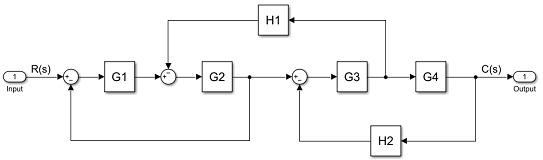
Figure 2 Feedback-system block diagram

a. Using Mason's gain formula, derive the closed-loop transfer function T(s) for the system with three overlapping negative-feedback loops shown in Figure 2.

T(s) = C(s) = ∑iPiΔi

R(s) Δ

Using two locations after the summing points with lower case e and a, apply block reduction method to derive the closed-loop transfer functions C/R and C/L for the system shown in Figure 3. The result should be a rearrangement to get C out explicitly.

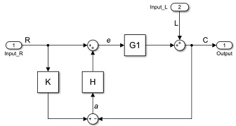
Figure 3 Feedback-system block diagram

QUESTION 4

Consider the radar dish motor control system block diagram shown in Figure 4. A proportional controller is required to yield a 20% overshoot (±1%) in the transient response for a unity step input.

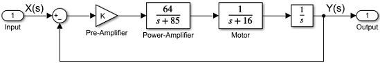
Figure 4 Radar dish motor control system

a. Calculate the damping ratio using the formula below.

ζ = -ln(%OS/100)/√(Π² + ln(%OS/10)²)

b. Calculate the phase margin using the formula below, your answer should be in degrees.

PM = tan-1 2ζ/√-2??² + √1 + 4??4 (rad/s)

Find the value of K that will yield a 20% overshoot (±1%) in the transient response for a unity step input.

Using MATLAB instructions, show the closed-loop feedback system response to a unity step input yields a 20% overshoot (±1%).