THE MODEL BUILDING 

A model of individual or aggregate economic phenomena represents a simplification of real world economic complexities. It may be expressed in words, tables, graphs, and mathematical equations. By inferring from detail and focusing attention on the essential relationships a model simplifies reality so that we can understand it properly.

Economic theory or models are often criticized as unrealistic. However it should be kept in mind that the world is too complex to be described in complete detail. The adequacy of the economic theory or model should, therefore, be judged in terms of their explanatory power rather than their realistic detail.

If we look at the development of macroeconomic analysis, the salient feature is the macroeconomic model of the economy that began with the classical model of pre-keynesian economic theory. Subsequently, almost all major developments in macroeconomic analysis were conveniently absorbed into this model as refinements or new additions. Keynesian theory was considered as an attempt to make the model more general compared to the classical model.

The analysis of monetary and fiscal policies is most successfully conducted within the framework of the model, and the monetarist-fiscalist debate cannot be unravelled without this model. The model has always had a demand side and a supply side. Keynes' emphasis on demand did not reflect ignorance of the supply side but rather came in response to the problems that were most pressing in his time. Similarly, concern with supply issues in the 1970s did not mean that demand economics was obsolete. For sometime insufficient attention had been paid to the supply side and that the supply components of the model were in need of sharpening. Finally, inflation meant that ways had to be found to replace the price level on the axis by the inflation rate and that the analysis had to be directed toward how the economy behaves when it is in a state of constant disequilibrium.

When the aggregate demand and supply model is drawn as a picture, it looks very much like a supply-demand diagram describing conditions in a market for a single commodity. In such a representation, price is posted on the vertical axis and quantity on the horizontal. In the aggregate demand and supply diagram, the overall level of prices is measured vertically, while total production (real national income) is measured horizontally. 

Although representations of aggregate demand and supply have the same general appearance as the demand-supply diagrams used in micro theory, there is a world of difference. Aggregate demand, for example, is the end result of all the factors that determined the level of total spending by consumers, investors, government, and foreign countries. It is influenced by countless factors, including the money supply and interest rates, taxes and government spending, international rates of currency exchange, and expectations of inflation. In fact, aggregate demand is such a vast subject that the bulk of most macroeconomics textbooks is devoted to it. 

                                                                                                      Figure 2.2                                                                

Similarly, aggregate supply is a complex relationship that is determined by technological factors, the supplies of capital and labor, the behavior of labor markets, pricing decisions by business, and again, expectations of inflation.

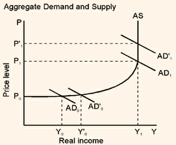
Different approaches to policy can be explained with reference to aggregate demand and supply even though we do not know yet how to derive these curves. Consider Figure 2.2, which shows an aggregate supply curve. It has a horizontal segment that generally is associated with deep recession or depression, a vertical segment that generally is associated with the classical full-employment economy, and an intermediate range that is upward-sloping. The equilibrium output and price levels are established at the intersection of the aggregate demand and supply curves. Expansionary monetary and fiscal policies generally raise aggregate demand. If the intersection is in the vertical range at P1 and Y1, an increase in aggregate demand to AD1 is of no value since it fails to raise output permanently and thus its effects are frittered away in higher prices. If aggregate demand is vertical, there is no point in having monetary policy and fiscal policy.

By contrast, suppose aggregate demand cuts aggregate supply in the horizontal range at Po and Yo. Here an increase in aggregate demand to ADo raises output without affecting prices at all. In such a situation monetary and fiscal policies can be used to take advantage of a slack in the economy to raise both production and employment without creating concern about inflation. 

                                                                                        Figure 2.3 

It is indicative that the shape of the aggregate supply function is critical to any intelligent discussion of the effectiveness of demand management policies because it is aggregate supply that determines the proportions in which an increase in aggregate demand raises output as opposed to prices.

What policy options are associated with monetarism and fiscalism within this model? If you believe that fiscal policy is ineffective but that monetary policy is effective, you will have to show that aggregate demand can be shifted only by means of monetary policy. If you believe that monetary policy is ineffective, you must show that an increase in the money supply will not affect aggregate demand but that fiscal policy will. These two situations represent two extremes and obviously have their own limitations.

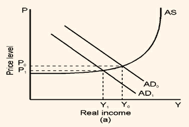
The different impact of shocks from both the demand side and the supply side is shown in Figures 2.3a and 2.3b respectively. In Figure 2.3a we imagine that output and prices fall from Yo to Y1 and Po to P1, respectively, in response to a reduction in aggregate demand. Such a reduction may come about because of a decline in foreign demand for our products or because of a reduction in capital (investment) spending resulting from a lull in inventive activity. The appropriate policy response is to offset the demand shock through an increase in demand by means of fiscal policy, monetary policy, or both. Thus the role for policy seems clear. Even with limited knowledge it seems reasonable to follow the rule that a demand disturbance should be offset by a demand management policy.

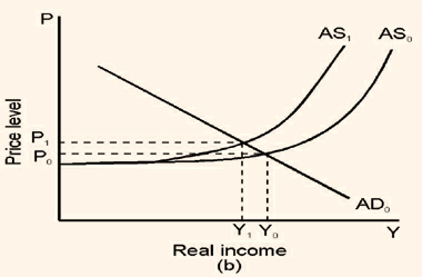
For example the price of imported oil rises. Because the cost of production of energy-using firms increases, they will have to be compensated for the increase by higher product prices in order to maintain existing production levels. As shown in Figure 2.3b, this means higher prices at all output levels, which implies a shift to the left of the aggregate supply curve. The shift causes output to fall from Yo to Y1 as in the case of the demand shock, but now the price level rises instead of falling. 

What will be the response of the policy? If we are accustomed to using only demand management, we quickly find ourselves in a dilemma. If we restore the existing level of production, we will have to use expansionary policies to raise aggregate demand to the point where it cuts the new aggregate supply curve at Yo. But this will add still further upward pressure on the price level. Conversely, if we want to hold the line on prices, we will have to reduce aggregate demand so as to cut AS1, at the original price level, Po. But this will cause output to contract still further.

Here the policy option is to look for those alternatives which can offset a possible disturbance and counter the supply shock effectively. The appropriate policy initiative is to deal with the oil shock at the source by finding a way to prevent OPEC decisions from influencing the domestic price of oil, or failing that, finding offsetting ways to shift aggregate supply to the right. This may involve tax policies that restore work incentives, policies that raise investment and increase the stock of capital, and various other supply-side measures.