Reference no: EM13835352
Background info:
Flows around cylinders of various cross-sections continue to engender a significant amount of engineering research interest due to its ubiquitous nature in society. Examples include bridge spans and pylons, high-rise buildings, pipelines, heat exchangers and oil platforms. When fluid (such as air or water) flows around such bodies, a wake develops which may become unstable and lead to a development of vortex streets. An example of the vortex street formed by clouds flowing past an island is illustrated in Figure 1.
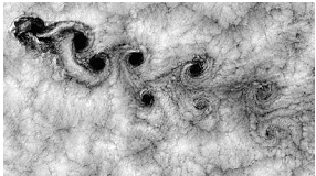
Figure 1. Kármán vortex street caused by wind flowing around the Juan Fernández Islands off the Chilean coast.
The vortices that develop are capable of containing large amounts of energy which can cause damage to neighbouring structures on impact. Therefore engineers and scientists study the wake dynamics behind these bodies with the aim of determining when such a flow transitions from a laminar state to a vortex-shedding state. This transition point is known as the critical point. In controlled environments, engineers are able to suppress or encourage vortex shedding depending on the purpose of the application. Thus it is crucial to determine the critical point. An example of where vortex shedding is encouraged involves using the vortices to dissipate heat from a heated wall (components in a computer).
A non-dimensional parameter commonly used to characterise this type of flow is given by the Reynolds number, Re. The Reynolds number describes the ratio between inertial to viscous forces. That is, a small Reynolds number flow is typically laminar as it is dominated by viscous forces. Increasing the Reynolds number increases the susceptibility to vortex shedding in the flow.
An engineer has performed experiments in a water channel involving flow past a triangular prism. Contours of axial vorticity at a low Re flow (Re=32) and a high Re flow (Re=50) are shown in figure 2 for visualisation purposes. It is clear that the flow transitions from a laminar to a vortex-shedding state somewhere between Re=32 and Re=50. The decay of the amplitude of the lift force signal when the Reynolds number was decreased from Re=50 to 4 different Re cases (Re=32, 34, 36 and 38) are recorded in the text files provided. The engineer is a little clumsy and cannot find the lift force data for Re=50 but knows for certain that it was a vortex-shedding state from the visualisation images.
The text file for each Re case contains:
1. The time, t
2. The amplitude of the lift force, A
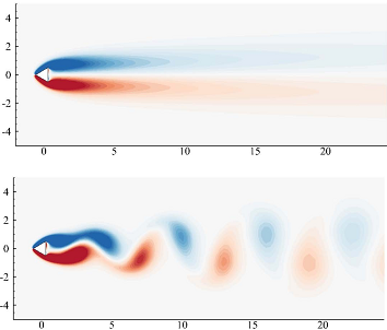
Figure 2. Axial vorticity contours of flow past a triangle oriented at 0? for Re=32 (top) and Re=50 (bottom).
The lift force amplitude information can be used to predict the critical Reynolds number which describes the point of transition from laminar to vortex-shedding flow.
In determining the critical Reynolds number, the engineer has asked you to perform the following tasks.
Q1a.
In the q1a.m file, read in the data for Re=32, 34, 36 and 38. Be aware that there is header information. Create a single figure with four sub-plots in a 2-by-2 arrangement. Plot the amplitude against time for each Re in each sub-plot window. The plot characteristics for all four sub-plot windows should be a black continuous line.
The title of your sub-plot windows should correspond to the Re of the data.
Q1b.
In reviewing the plots created in Q1a, you notice that the lift force amplitude obeys an exponential relationship. That is, the lift force amplitude could be described by
A = αeβt
where α and β are constants.
In the q1b.m file, you are required to create another single figure comprised of four sub-plots in a 2-by-2 arrangement. Now plot the linearised lift force amplitude against time for each Re in each sub-plot window.
The plot characteristics for all four sub-plot windows should be a red continuous line. The title of your sub- plot windows should correspond to the Re of the data.
Q1c.
You have shown the engineer plots you created in Q1b. The engineer notices that the data becomes consistently noisy after a certain amount of time for each Re data set. Also, the lift force ultimately becomes constant as the apparatus used to measure the lift force is unable to measure smaller amplitudes. Therefore, the engineer believes that data beyond t=350 for Re=32 should be removed.
In the q1c.m file, you are required to remove the consistently noisy data for each Re data set. The threshold for when the consistently noisy data differs for each Re set. Use the probe tool to estimate where the data begins to become consistently noisy. Do not use NaN.
In a new figure, recreate the plots from Q1b but now plot the linearized lift force amplitude against time without the consistently noisy data. The plot characteristics for all four sub-plot windows should be blue circles. The title of your sub-plot windows should correspond to the Re of the data.
Q1d.
The engineer would now like to see how well the noiseless data conforms to the exponential relationship proposed in (eq. 1). Therefore, the engineer wants you to curve fit the noiseless data you've just plotted in Q1c.
In the q1d.m file, use polyfit to determine the constants α and β in (eq. 1) and therefore the nonlinear equation. Determine the nonlinear equations for all four Re cases. Use the fprintf function to print the equation for each Re and the corresponding coefficient of determination, r2. Use 4 decimal places for the α and β constants and 6 decimal places for the r2 values.
On the same figure created in Q1c, plot the fitted curve to each Re data set. The plot characteristics of the fitted line should be a green continuous line with a line width of 3. The title of your sub-plot windows should be updated with the corresponding Re and nonlinear amplitude equation. Place a legend in the bottom-left hand corner of each sub-plot.
Q1e.
It turns out that the β constant in (eq. 1) corresponds to the growth rate of the wake. Negative growth rates represent a weakening oscillation signal towards a steady/laminar flow state, while positive growth rates indicate that the oscillations become stronger towards/past a vortex-shedding flow. Thus, a growth rate of zero is of interest as it corresponds to the transition between laminar to vortex-shedding flow. This flow is known as the critical Reynolds number flow. The engineer wants you to use polyval to curve fit the β against Re data to determine the critical Reynolds number using a range of polynomial degrees. The polynomial degrees range from linear to a maximum degree which is specified by the user.
In the q1e.m file, plot growth rate against Re using magenta diamond markers. Starting from a linear polynomial degree, fit the data to determine the critical Reynolds number (where the growth rate is equal to zero) using a closed root-finding method. Continue to increase the polynomial degree up to a user-specified number. For example, if a user inputs a maximum degree of 4: you will determine the critical Reynolds numbers using a linear fit, parabolic fit, cubic fit and quartic fit.
On the same figure of the magenta diamonds, plot the fitted polynomial curve using a continuous black line and mark the critical Reynolds number and corresponding growth rate with a red asterisk. For example, a maximum degree of 4 will have four critical Reynolds numbers and therefore should have 4 red asterisks. In additional, plot a solid-filled green diamond of marker size 10 to represent the mean critical Reynolds number calculated.
The title of the plot should display the mean critical Reynolds number. Place a legend in the top-left hand corner of each sub-plot. The green diamond does not need to be included in the legend. That is, only the ‘data', ‘fit' and ‘roots' need to be in the legend. In addition, use fprintf to print the mean critical Reynolds number to the command window.
Prompt the user as to whether or not they want to repeat this section of code (Q1e) so that a new maximum polynomial degree can be inputted. Continue to do so until the user decides to stop.
QUESTION 2
A free-swinging pendulum with damping is modelled using the following equation:
d2θ/dt2 + c/m. dθ/dt + g/l sin(θ) = 0
The constants in the equation are:
Damping coefficient: c = 1 s-1
Mass: m = 1 kg
Gravity: g = 9.81 ms-1
Link length: l = 0.5 m
Given the initial conditions, θ(0) = 90° and θ'(0) = 0, solve this equation from t = 0 to t = 10 with a interval of 0.01s using
• Euler's method
• Heun's method
• The 4th order Runge-Kutta method
You will need to write your own code to use the Euler, Heun's and Runge-Kutta formulae. Please answer the following questions in the q2.m file:
a) Plot the angle of the pendulum as calculated from all three ODE solver methods on a single plot, ensuring that the plot is titled, all axes are labelled, units are indicated, and the legend for each solver displayed in Best configuration.
b) Plot the angular velocity of the pendulum for each solver using subplot(), where all plots are stacked vertically in the figure such that the x-axes are lined up. Annotate all plots accordingly.
c) Without plotting, what will happen to the pendulum if no damping was present? (i.e. c = 0). Answer using the fprintf command.
d) Repeat a), but with the damping coefficient set to 0.
• Is the result what you expected from your answer in c)?
• Why does the Euler method (and to a certain extent, Heun's method) give this result?
Comment on the solver's accuracy and give a possible reason as to why this occurs in this particular initial condition. Answer using the fprintf command.
QUESTION 3
Melbourne's water supply network consists of a network of dams and reservoirs that store water from water catchments, situated all around Victoria. These catchments catch rain water and transport them via pipelines to the nearest reservoir. One of the main reasons for storing this water is to safeguard us against drought, so we may continue to use water while we wait for the next rain event to fill our dams. However, the effects of climate change have had severe effects on water storages. In this exercise, we will use water storage data provided by Melbourne Water1 to visualise how our water storage levels have changed since 1940.
Expressed as a % of the total capacity of the storage network, the data is stored in a csv file in monthly intervals, beginning from January 1940 to August 2015.
Q3a.
Write an M-file that plots the water storage level data between a specified month and year. In order to complete this task, you need to use the m-file provided to you, called q3a.m. This file is partially complete, and you will need to complete and/or answer the following sub-tasks to complete this question.
i. Fill in the code to read the csv file using importdata(). The water level data should be stored in a variable called WaterLevel, and string data for year called StrYear and string data for month called StrMonth. You may need to trim the top string entry in textdata using (2:end) if needed.
ii. Fill in the code to prompt the user to enter the starting year and month and the ending year and month to plot. Name the start year and month y1 and m1 respectively, and end year and month y2 and m2 respectively. The month entered should be entered as a number between 1 and 12.
iii. Notice that the first data entry is for January 1940 in which the dams were 87.62% full is stored as WaterLevel(1). Because the data is stored monthly, this means that the index represents the number of months since January 1940, and as such, WaterLevel(13) is the water level January 1941 and so on. If we want to get the water level at January 2000 for example, we need to convert a year and month entry to the proper array index. In the section provided in function getarray(y,m), write the equation that converts year and month to an array index.
iv. Utilising the function getarray(y,m), plot the water level data between your specified dates, where xData represents your x-axis.
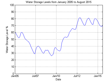
v. You can now run your code now to check if it plots correctly. If it works, then you can start formatting the plot so that the data presents better. Using an example plot below where data is plotted between January 2005 and August 2015, run enter the code in the provided section to get the required labels on the plot:
• Label x and y axes (x-axis dates are already provided)
• The title of your plot should change depending on which period you choose. If you plot from January 1940 to January 2015, then the title must say "Water Storage Levels from January 1940 to January 2015". You may use sprint(), along with StrYear{} and StrMonth{} for this, i.e. StrYear{1} = ‘1940', StrMonth{1} = ‘January'.
• The grid should be on and the y-limits should be from 0 to 100%
Q3b.
If you were to plot the entire data set from 1940 to 2015 (1941,1,2015,8), the plot is very difficult to read due to the high number of data points. In order to observe longer term trends within the data, we should interpolate it by fitting a polynomial to it. Using the provided M-file q3b.m, fit a 12th order polynomial to the data. Plot the original data and the 12th order polynomial in the same plot. The polynomial line should be of width 2 and in red. You may ignore any warnings generated by polyfit().
Q3c.
Using the results generated from Q3b, write code in q3c.m to find:
i. The lowest water level on record, along with the month and year. Mark this in the plot generated in Q3b with a red square marker that is outlined in black, size 10.
ii. The highest water level on record, along with the month and year. Mark this in the plot generated in Q3b with a green diamond marker that is outlined in black, size 10.
Use fprintf() to display this information in the command window in sentence form. E.g.
The lowest water storage level is X1% in month Y1, year Z1.
The highest water storage level is X2% in month Y2, year Z2.