Carnot Cycle

The Carnot's principle is best elaborated with a simple cycle as shown in figure below and an illustration of a proposed heat power cycle. The cycle consists of the reversible procedures shown below.

1-2: adiabatic compression ranges from T_C to T_H due to the work executed on fluid.

2-3: isothermal expansion as fluid expands whenever heat is added to the fluid at temperature T_H.

3-4: adiabatic expansion as the fluid executes work during the expansion procedure and temperature drops from T_H to T_C.

4-1: isothermal compression since the fluid contracts whenever heat is eliminated from the fluid at temperature T_C.

This cycle is termed as a Carnot Cycle. The heat input (Q_H) in a Carnot Cycle is graphically symbolized on figure shown below as the region under line 2-3. The heat rejected (Q_C) is graphically symbolized as the region under line 1-4. The difference among the heat added and the heat discarded is the net work (sum of all work procedures), that is symbolized as the region of rectangle 1-2-3-4.

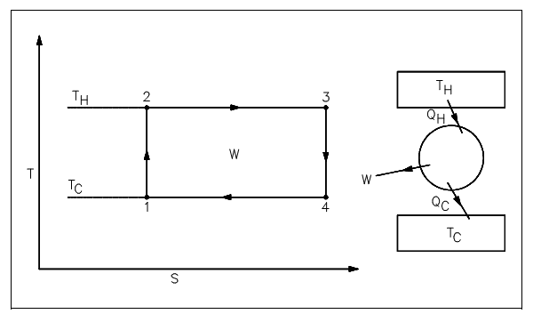
Figure: Carnot Cycle Representation

The efficiency (η) of the cycle is the ratio of the total work of the cycle to the heat input to the cycle. This ratio can be stated by the following equation.

η = (Q_H -Q_C)/Q_H = (T_H -T_C)/T_H

= 1- (T_C/T_H)

Here:

η = cycle efficiency

T_C = designates the low-temperature reservoir (°R)

T_H = designates the high-temperature reservoir (°R)

Equation above shows that the maximum probable effectiveness exists whenever T_H is at its largest possible value or whenever T_C is at its smallest value. As all practical systems and procedures are really irreversible, the above effectiveness symbolizes an upper limit of effectiveness for any given system operating among the similar two temperatures. The system's highest possible efficiency would be that of Carnot efficiency, though since Carnot efficiencies symbolize reversible processes, the real system will not reach this efficiency value. Therefore, the Carnot efficiency serves as an unachievable upper limit for any actual system's effectiveness. The illustration below explains the Carnot's principles.

The most significant aspect of the second law for our practical reasons is the determination of maximum possible efficiencies acquired from a power system. The real efficiencies will forever be less than this maximum. The losses (friction, for illustration) in the system and the fact that systems are not truly reversible prevent us from acquiring the maximum possible effectiveness. The example of the difference that might exist among the ideal and real effectiveness is presented in figure shown below.

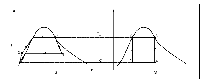
Figure: Real Process Cycle as Compared to Carnot Cycle

An open system analysis was performed by using the First Law of Thermodynamics. The second law problems are treated in much the similar way; which is, an isolated, closed, or open system is employed in the analysis based upon the kinds of energy that cross the boundary. Since with the first law, the open system analysis by using the second law equations is more common situation, with the closed and isolated systems being "special" situations of the open system. The answer to second law problems is very similar to the approach employed in the first law analysis.

The figure below illustrates the control volume from the point of view of the second law. In this diagram, the fluid moves via the control volume from section to section out whereas work is delivered external to the control volume. We presume that the boundary of the control volume is at some atmospheric temperature and that all of the heat transfer (Q) takes place at this boundary. We have noted that entropy is a property; therefore it might be transported with the flow of the fluid into and out of the control volume, just similar to enthalpy or internal energy. The entropy flow in the control volume resultant from mass transport is, thus, m_ins_in, and the entropy flow out of the control volume is m_outs_out, supposing that the properties are uniform at sections in and out. Entropy might also be added to the control volume since of heat transfer at the boundary of the control volume.

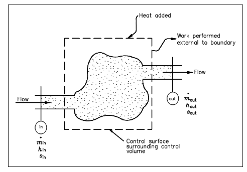
Figure: Control Volume for Second Law Analysis

A simple elaboration of the use of this kind of system in second law analysis will give the undergraduate a better understanding of its utilization.