Utility Maximisation:

Graphical Presentation 

Let consider a two-commodity world, x₁ and x₂ representing good I and good II respectively. p₁ and p₂ are the prices of good I and good II respectively, where the prices are given to the consumer, i.e., prices are exogenously given and consumer can't change them. Money income of the consumer is M, which is also exogenously given to the consumer. Note that p₁x₁+p₂x₂ is the total expenditure of the consumer when she consumes x₁units of good I and x2 units of good two. The total expenditure of the consumer can't exceed her money income, therefore  p₁x₁ + p₂x₂ ≤ M  ------- (a)  

Equation (a) is known as consumer budget constraint. Let U = U(x₁, x₂) is the utility function of the consumer. Therefore, consumer must solve the following Maximisation problem(UMP):   

As consumer objective is to maximise her utility and as larger consumption leads to larger utility, she always wants to consume more of any goods. But she also has to spend some amount of her income to consume larger amount of goods. So ultimately in equilibrium she will spend all her income and M = p₁x₁+p₂x₂.  

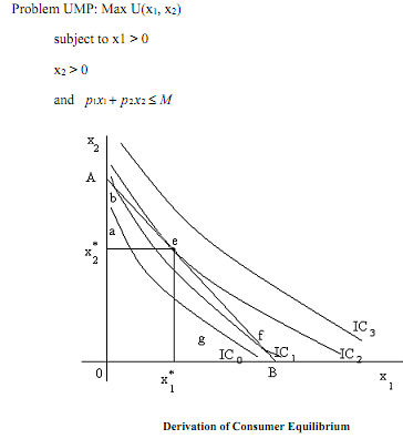
Consumer Behaviour  Now suppose that the line segment AB represents the budget line. Along AB p₁x₁ + p₂x₂ = M  holds. Let initial indifference curve of the consumer is IC0. In IC0, there are many points along that indifference curve such that p₁x₁ + p₂x₂ ≤ M holds. Therefore, utility maximising consumer will spend more as she moves to higher indifference curve (say IC₁). In IC₁ there are still such points along the indifference curve such that p₁x₁ + p₂x₂ ≤ M  holds, so again consumer spends more. This process will continue as long as consumer reaches an indifference curve where for no point along the indifference curve p₁x₁ + p₂x₂ ≤ M holds and at least one point of the indifference curve is on the budget line. At that point, we have consumer equilibrium, C(x₁, x₂) = (x₁*(M,p₁,p₂), x2*(M,p₁,p₂))(in Figure point 'e' is the equilibrium point). Not that at equilibrium, slope of the indifference curve is equal to the slope of the budget line. Therefore, at equilibrium we have 

1) Budget constraint holds with equality sign. 

2) Slope of the indifference curve is equal to the slope of the budget line.