In Time Series Analysis, we try to identify and determine the pattern of changes in the data collected over regular intervals of time. The data collected can be at a periodical interval of days, weeks, months and years. After identifying the patterns, we project them into future to get an estimate of the variable under consideration. Do the changes or variations observed in different time series be the same or different? Necessarily, they should be different as the independent variable (X) on the axis which influences the dependent variable differs from one time series to another. Broadly, the variations observed in time series can be classified as (i) the secular trend (ii) the cyclical fluctuation (iii) the seasonal variation and finally (iv) the irregular variation. We will look at each of them. 

Secular Trend

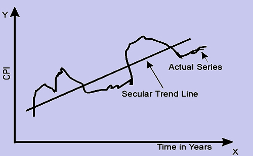
Under this type of variation, we look at the long-term behavior of the variable. This is important in the sense that one should be able to conclude whether the value of the variable has been increasing or decreasing over the years, keeping aside the variation observed in the individual years which constitute the series. An appropriate example of secular trend would be the variation in the Consumer Price Index (CPI) observed over a period of say 20 years. The Secular Trend can be represented graphically as shown in figure 1. In the figure, the secular trend is shown as a straight line, with an upward slope, while the actual time series is shown as a curve moving towards and away from the trend line.

Figure

The next logical question would be, apart from deciding the long-term trend of the variable, what are the other advantages of studying the secular trend? They can be listed as:

1. By studying the secular trend one can examine whether a policy implemented has yielded the necessary results or not and what would be its future impact.

For example, if a decision is taken to introduce multiple quality checks for a product, then it is possible to use the secular trend in the past to verify whether the decision resulted in significant reduction in poor quality products getting into the market. Similarly, if a department is constituted to follow the receivables of a company, it is possible to see whether this measure has resulted in any improvement in the recovery of receivables.

2. After studying the secular trend, one can project it into the future to get an estimation (future value) of the variable. This helps us to take necessary measures in time.

A secular trend gives us an understanding about the behavior of a variable. Hence it will be possible to project its value to a future date to know what the value is likely to be. For example, a company which proposes to develop a medium-term plan can have a sales forecast based on the historical trend.

3. Under certain circumstances, it is required to examine the time series for other variation components only. Therefore, by studying the secular trend one can separate it, which in turn facilitates the study of other components present in the series.

While studying the trends in inflation it is possible to study the impact of seasonal variations for which separation of the impact of secular trend is necessary.

In the figure above, we have seen that the secular trend is a straight line. Do all the trend lines need to be linear? No, it is not mandatory that all the trend lines are to be linear in nature. It depends on the phenomena which we are trying to explain. This is because, some relationships are amenable to be dealt by using linear (straight line) models, while the characteristics of some others can be better brought out and examined if we use a curvilinear model. For example, the pollutants in the environment do not increase in a linear fashion. In this case, a curvilinear model may be more appropriate as compared to a linear model. Can we fit the trend, whether it be straight line or curvilinear only by inspecting the points visually or follow a scientific procedure? Yes, we can fit a trend observing the points visually. However, the problem with this method is that different people tend to have their own bias giving rise to ambiguity. Therefore, to get a best fit, we employ the least squares method, which we have first seen in Linear.

 

1. The equation of a straight line is given by Y = a + bX, where X and Y are independent and dependent variables, "a" is the Y-intercept (the value of Y when X is equal to zero. That is Y = a + b.0 = a + 0 = a) and finally "b" is the slope of the straight line.

2. For the given values of X and Y, we run regression analysis to get the estimating equation, which is of the form = a + bX. At this point, it is worthwhile to note that the general trend of the given time series can be expressed in terms of any number of straight lines. But what we are concerned is with the straight line which is the best fit. That is, the deviations of the actual series and the estimated points, when squared and added should give a value, which is minimum if we repeat the process for other straight lines obtained from the given data. This can be achieved if we employ the equations for "a" and "b" given below.

 

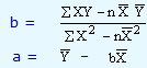
where "a" and "b" are the Y-intercept and the slope of the estimating equation, "n" is the number of data points in the series,    and    are the mean values of X and Y data points.

We deal with the curvilinear trend later.

Since in time series, the independent variable X in most of the cases happens to represent years (2000, 2001, 2002,.....), our computational part will become tedious if we use it as it is. In order to make it easier, we take the mean of the X data points and subtract it from actual X values and represent that column as "x". This process is referred to as Coding or Translating time. Therefore, when there are odd number of data points, the middle point will become zero. When there are even number of data points, the mean will be like. 2001.5 This requires that after subtracting the mean from the actual data points, we multiply the resultant values with 2 and denote that column as "x". In other words, "x" denotes the coded time in terms of half year intervals. The other advantage of this process is that, the value of the mean happens to be zero. Incorporating these changes in the equations for "a" and "b", we get

b =

and a =