As we know that price of option-free bond changes in the opposite direction from a change in bond's required yield, Table 1 and figure 1 explains this feature of option free bond.              

Table 1: Relationship of Price/Yield for Six Hypothetical Option Free Bond  

* Prices = Coupon Income x PVIFA_{(Kd, n)} + Par Value x PVIF_{(Kd, n)}

All the values are computed in the similar maner.

We can see that value of long-term bond (20-years bond) decreases faster than short-term bond (5-years bond). 

Figure 1: Price/Yield Relationship for a Hypothetical Option-Free Bonds

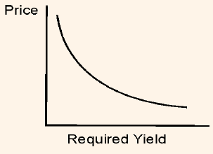
It is very clear from the chart that with every increase in the required yield, price of option free bond decreases. We can also notice from the chart that the price/yield relationship is not linear. The shape of line representing the relationship of these two is known as a convex.

We can measure the rupee price or the percentage price change in the bond price due to change in yield. Table 2 shows the percentage change in the bond prices given in Table 1 due to various changes in yield.

Table 2: Instantaneous Percentage Price Change for three Hypothetical Bonds

A critical examination of Table 2 reveals the following properties concerning the price volatility of an option-free bond:

Property 1: Price moves in the opposite direction from the change in required yield. However, the percentage change in the price is not same for all bonds.

Property 2: The small changes (increase or decrease) in the required yield are roughly same to the percentage price change from a given bond.

Property 3: When the change in the required yield is large, the percentage change for an increase in required yield differs from the percentage price change for a decrease on the required yield.

Property 4: The percentage price increase is greater than the percentage price decrease for a given large change in basis points in the required yields.

Though the properties are expressed as percentage price changes, it is true even for the rupee price changes.

Let us explain Properties 3 and 4 with the help of Figure 2.

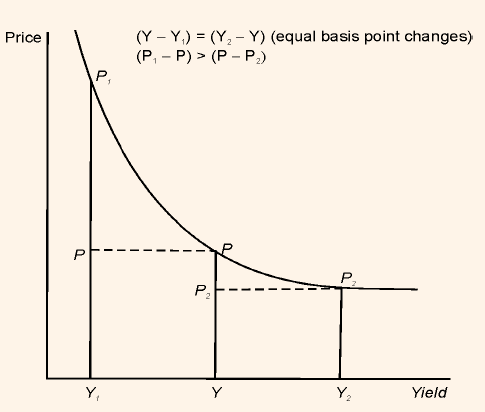
Figure 2: Graphical Representation of Properties 3 and 4 for an Option-Free Bond

In Figure 2, horizontal axis represents the yield and vertical axis represents the Price of the bond. In addition, Y, Y₁ and Y₂ represent the initial yield, lower yield and higher yield respectively. In the same way, P, P₁ , and P₂ represent initial price, price at lower yield and price at higher yield respectively. The initial yield decreases and increases in such a manner that,

         Y - Y₁ = Y₂ - Y

Let us assume that there is a large change in basis points in the required yield.

When yield increases from Y to Y₂ then change in initial price (P) is equal to the difference between the new price (P₂) and the initial price. That is,

         Change in price when yield increases = P - P₂

When yield decreases from Y to Y₁ then change in initial price (P) is equal to the difference between the new price (P₁) and the initial price. That is,

         Change in price when yield decreases = P₁ - P

We can see from the chart that the change in price when yield decreases is not equal to the change in price when yield increases. That is,

         P₁ - P ≠ P - P₂

Property 3 states the same point. In addition, when we compare the price change in both situations, then we find that the change in price is greater when yield decreases than when the yield increases. That is,

         P₁ - P > P - P₂

Property 4 states the same point. This property implies that when an investor in bond holds a long position, the price appreciation an investor would realize from the decrease in the required yield would be greater than the capital loss that he would realize when there is a decrease by the same number of basis points in the required yield y. For an investor holding a short position in bond, the opposite would be true. That is, the potential capital loss is higher than the potential capital gain if yield changes by a given number of basis points.

Now let us understand how the convexity of price/yield relationship impacts Property 4. Figures 3 and 4 graphically explain the impact.

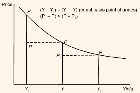
Figure 3: Impact of Convexity on Property 4: Less Convex Bond

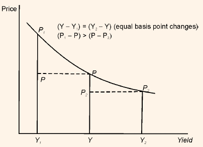
The Figure given above is showing a less convex price/yield relationship than figure 2. Let us see the impact due to the difference in convexities, i.e., when the yield increases and decreases by the same number of basis points and yield change is a large number of basis points. In figure 3 we notice that while the price gain when the required yield decreases is greater than the price decline when the required yield increases, there is not much difference in the amount of gain and amount of loss, or in other terms the gain is not much greater than the loss. But in figure 4 we see that the bonds have greater convexity than the bonds in figure 3. We can notice that the price gain is much greater than the loss.

Figure 4: Impact of Convexity on Property 4: Highly Convex Bond