Bond management evolution to some extent is linked to the increased volatility of the interest rate term structures which is in existence since seventies. Bond valuation can be better understood by understanding the determinants of default risk, of liquidity premia and of tax advantages that are linked to current yield. The wider use of sophisticated bonds with call or put options, sinking provisions and uncertain cash flows are proving complicated to the bond investor. Hence, building of MFMs for bonds has provided the required tools for better control of risk in bond management.

Model Specification

Model Specification can be discussed in the following manner:

• The Single and Two Factor Duration Models: The duration concept can be taken as a crude but nevertheless powerful single risk factor model. Let us consider that for small changes in the level of interest rate, we have:

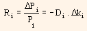
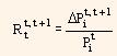
In the above equation, R_i represents return of bond i, P_i represents price of bond i, D_i indicates modified duration of bond i and k_i represents yield of bond i now (YTM). This equation can be used for instantaneous change in yield and also as proxy for a short period of time. Then, the equation can be written as

         Where,

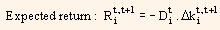
                       represents return to bond i during time period t to t + 1.

Here, we again find a predictive model that relates to the volatility of a bond return to the volatility of its current yield, the proportional coefficient being the bond duration. This can be stated as a simple single factor mode wherein the duration of a bond is its factor exposure. This model assumes that the term structure is flat and considers only small parallel shifts.

The quality of the forecast can be improved by considering convexity, in order to predict price changes in bonds for parallel shifts in term structure. This can be shown by the following equation:

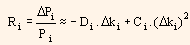
Here, C_i  represents convexity of bond i.

      This can be said as a two factor model as duration and convexity of bond become its factor exposures. This model also relies on the same simplistic assumptions of term structure and its movements.

• The Full Term Structure MFM: Let us consider a better description of the movements in the term structure in interest rates so that the deficiencies in the earlier approaches discussed above can be corrected. Let us begin with the conventional evaluation of a bond model:

                                                                                                ... (1)

 Proxy implies an approximation as interest accrual is ignored and an assumption is made that the duration is constant through time.

Here,

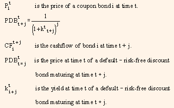
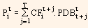
While using the above formula, the yields of the discount bonds need not be identical for different maturities. This facilitates us to incorporate more complex interest rate term structures and their realistic movements. By using equation (1) we get instantaneous movements in the discount rate term structure. If we extend it as a proxy for price variations through small time periods, we get:

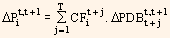
By dividing the above equation by the price of the bond and after certain manipulations we get:

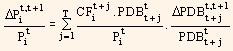
If we introduce some new notations, the above equation can be written as

                                                          ... (2)

Where,

is the return of the bond i between t and t + 1.

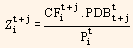
is the fraction of the value of the bond i related to cash flow t + j.

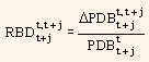
is the return of the default-risk free discount bond maturing at t + j between t and t + 1.

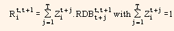
From equation (2) it can be said that the return of a bond is a weighted average of the return of the zero-coupon bonds. In case we consider the zero-coupon bonds as factors, then, the bond exposure on them will be the fraction of its value that is related to the cash-flow of the same maturity as the zero-coupon bond.

Suppose we assume a set of predetermined set of discount maturities as given in the following table:

Table 4

Through the above set of predetermined discount maturities, we can summarize for each bond i its exposures to all zero-coupon bonds in the form of a vector notation:

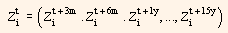
Using above equation and covariance matrix W (given) for the returns of the set of zero-coupon bonds, the variance of the return of bond i can be presented in the following way:

represents the variance of the return of bond i between time t and time t + 1. This forms the foundation for a risk model. Both historical estimates as well as forecast of covariance matrix can be obtained from time series analysis of the factor returns. Thus, we now have a fully predictive risk model.

     However, this model is not limited to unrealistic assumptions of the shape and the movements of the interest rate term structure. It is also not convenient to use this model while implementing strategies for complicated movements in interest rate term structure. Such scenarios, to be translated into desired exposures for each discount maturity, need a sophisticated computer program.