The graphical method is a simple one, and is the most easily understood of the several linear programming methods. A thorough knowledge of the graphical procedure provides necessary insight and confidence to understand the more advanced methods and concepts behind these methods. However, it should be pointed out that the graphical method can be applied only in the case of two variables. It cannot be applied to problems with many variables.

Maximization

Example 

Consider a small foundry which specializes in the production of iron castings. For the sake of simplicity, assume that the foundry specializes in producing two types of castings - casting A and casting B. Because of a strong consumer demand for these products, it is assumed that the foundry can sell as many units as it produces. The profit is Rs.70 and Rs.40 for each of casting A and casting B respectively. The foundry manager should decide the quantity of these castings to be produced each week so as to maximize the total profit.

Production of castings requires certain resources like raw materials, labor and foundry capacity. The requirements and their availabilities are given in the following table:

Let us formulate this problem in terms of mathematical equations or inequalities.

As the manager has to decide the number of type A and type B castings to be produced, let us define the variables:

         q₁ = number of type A castings to be produced

         q₂ = number of type B castings to be produced

For this production schedule, the total profit will be

                   70q₁ + 40q₂

This function is known as the objective function which is to be maximized. If there are no constraints, the profit can be increased to infinity. In real life, there are restrictions of different kinds. These are formulated as constraints.

Let us consider raw material-1, of which only 120 kgs are available. If q₁ of type A castings and q₂ of type B castings are produced, then the requirement of raw material-1 is 2q₁ + 1q₂, and this should be less than or equal to the available quantity of raw material-1. This can be shown by the following inequation:

                   2q₁ + 1q₂ < 120

This implies that we are interested in the values of q₁ and q₂ for which the left-hand-side value is less than or equal to the right-hand-side value of 120. Otherwise, the requirement will exceed the availability and the production of that quantity will not be feasible.

By a similar argument, we get the constraints for raw material-2, labor and foundry capacity as:

         Raw material-2       :0.8q₁  + 0q₂ < 40

         Labor                   :3q₁ + 2q₂  < 200

         Foundry capacity   :4q₁ +  3q₂  <  360

As one cannot produce negative quantities, we have the restrictions:

         q₁ > 0, q₂ > 0

Putting together the above elements, the problem may be represented as:

Maximize Z: 70q₁ + 40q₂                  ....(1)

Subject to constraints:

    2q₁  +  q₂        <    120.

    8q₁   +   0q₂     <      40               ....(2)

    3q₁   +  2q₂     <     200

    4q₁   +  3q₂     <     360

      q₁ >0, q₂ > 0                            ....(3)

We have to find the values of q₁ and q₂ which will satisfy constraints (2) and (3) and at the same time maximize function (1). The function given in (1) is called an objective function. The inequalities in (2) are called constraints and the inequalities in (3) are called non-negativity restrictions or constraints. This problem cannot be solved by the calculus method because of the inequality constraints.

The first step in the graphical method of solution is to identify the region in the graph which corresponds to all pairs of values of q₁ and q₂ for which (2) and (3) are valid.

Let us consider the non-negativity restrictions given by (3). The values of q₁ and q₂ which satisfy these restrictions should fall in the first quadrant of the graph. Hence, We can ignore pairs of values of q₁ and q₂ which fall in other quadrants. This is indicated by arrow marks on the q₁-axis (or x-axis) and q₂-axis (or y-axis) in the graph shown below.

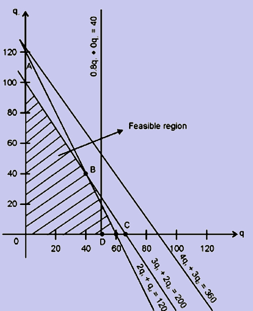
Let us next find the region corresponding to the values of q₁ and q₂ for which the first constraint

                   2q₁ + q₂ < 120

is satisfied. To do this, we have to first draw the line

                   2q₁ + q₂ = 120

For this, we need to fix two points on this line. The points that we have chosen are:

                   q₁ = 0                    q₂ = 120 and

                   q₁ = 60                   q₂ = 0

By joining these points, we get the line, and the points below the line, indicated by arrows, will satisfy the first constraint.

Other constraint equations are also drawn on the graph. The region common to all the regions identified gives the set of points for which the values of the co-ordinates q₁ and q₂ satisfy constraints (2) and (3). The region identified is OABCD is called the feasible region. It may be noted that all values of q₁ and q₂ which satisfy constraints (2) and (3), lie within the region OABCD and all points in the region OABCD will have the co-ordinates q₁ and q₂, which will satisfy constraints (2) and (3). Hence, an optimal solution to the problem should have co-ordinates q₁ and q₂ within or on the boundary of region OABCD.

Now let us search for the optimal solution.

Suppose, we are interested in finding a product mix which will give a profit of say, an arbitrarily chosen value of Rs.2,800. To get the product mix, we have to search in the region OABCD to examine whether any point gives a profit of Rs.2,800. The easiest way is to draw the straight line whose equation is

                   70q₁ + 40q₂ = 2,800

and examine whether it passes through any points in the region OABCD. In the graph given below, the feasible region OABCD and the above mentioned straight line are shown. We can observe that there are many points on this straight line which come under the feasible region, and each point will give the co-ordinates which refer to the production levels that yield the same profit of Rs.2,800. For example, take the two points (40,0) and (0,70) on this line. The production levels corresponding to these points are (i) 40 of type A castings and 0 of type B castings and (ii) 0 of A castings and 70 of type B castings. It can be verified that each co-ordinate gives the same profit. Thus, the straight line drawn is also the profit line.

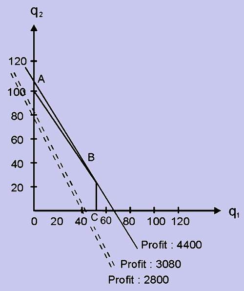
Suppose we wish to increase the profit, we look for a product mix which will give a profit of, say, Rs.3,080. As done earlier, we draw the line

                   70q₁ + 40q₂ = 3,080

and examine whether it passes through the region OABC. This line is parallel to the first line and passes through the feasible region, thus indicating that it is possible to increase the profit to Rs.3,080. This suggests that, as we move up this line in the Northeastern direction, parallel to itself, we can obtain product mixes which will give higher and higher profits. We should move the line as far as possible without removing it completely from the region of feasible solutions as otherwise we will not find any feasible product mix which will satisfy the constraints. The optimal solution is then given by the point of final contact, which will be one of the corner points. In this case, the point is B, whose co-ordinates are (40, 40), indicating that the production level should be 40 for each of type A and B castings and this will yield a profit of

         70 x 40 + 40 x 40 = 2,800 + 1,600 = Rs.4,400