Equilibrium Income 

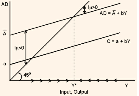
The next step is to use the aggregate demand function, AD, to determine the equilibrium level of income and output. This is done in figure . Recall that the equilibrium level of income is that level of income for which aggregate demand equals output (which in turn equals income). The   line which you see in the figure serves as a reference line that translates any horizontal distance into equal vertical distance.

Thus, anywhere on the   line, the level of aggregate demand is equal to the level of output. The level of income at which the aggregate demand line cuts the  line is the equilibrium income. We see from the figure that at an income level Y* the aggregate demand curve cuts the 45o. At Y*, aggregate demand is equal to income and thus is the equilibrium income and output. At any income level below Y*, firms find that demand exceeds output and that their inventories are declining. This unintended decline in inventories is shown as Im < 0 in the figure. In order to make up for the decline in inventories, firms increase production. Conversely, for output levels above Y*, firms find inventories piling up (Im > 0) and therefore cut production. As the arrows show, this process leads to output level Y*, at which current production equals planned aggregate spending and unintended inventory changes are equal to zero. Now, let us derive the formula for equilibrium output. At equilibrium, output is equal to aggregate demand. 

                                        Figure 4.3 

                 Y            = AD 

                     =       + bY 

          Y (1 - b)   = 

         Y  =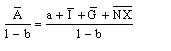

From the above equation we can see that the larger    is, (for a given b) the higher is the equilibrium level of income. That is, the larger the autonomous spending, indicated by   , the larger is the equilibrium level of income. Similarly, for a given   , the greater the slope (b) of the AD curve, the higher is the equilibrium level of income.