Classical Quantity Theories

Quantity theories have had a long history and a widespread use in economics. As originally formulated these were not explicitly designed as theories of demand for money but can be so interpreted.

The theory of demand for money has been derived from the 'equation of exchange' developed by Irving Fisher. Equation of exchange holds that the total amount spent by buyers equals the total amount received by seller. To state it mathematically,

MV = PQ = Y . . . .(A5.1)

M = Stock of money. It is simply the money supply i.e. total amount of money available in the economy.

V = Velocity. Velocity is the rate at which money moves as it carries out its functions. It is the number of times an average rupee changes hands during a period of time.

Or, in other words, it is the average number of times per year that each rupee of M is spent for output. For example, let us say that the following transactions took place during a year - Mr. A spends Rs.100 for a wrist watch. The shop owner uses it to pay wages to his clerk. The clerk pays Rs.100 towards his son's school fees. Thus, Mr. A's original Rs.100 has changed hands three times. Its velocity in terms of transactions is 3

        P       =       Price. It is the average price per unit of output or the price level of output.

         Q       =       Real output of goods and services.

         Y       =       PQ = GNP at current prices.

Thus, P x Q is simply the money value of all goods and services produced and sold. The right-hand side of the equation of exchange is simply the real flow (i.e. flow of goods and services), measured in money terms. The left-hand side is the money flow.

If Money Stock (i.e. M₃) is Rs.9,000 crore and each rupee averaged 3 trips around the circle each year, then the money flow would be Rs.9000 x 3 i.e. Rs.27,000 crore. Flow of goods and services (or GNP) would also be Rs.27,000 crore.

The other technique used to express the linkage between the stock of money and the flow of money expenditures is theCambridge approach which states that

M = kPQ = kY                                                                                               .....(A5.2)

where,

M, P and Q are defined as in equation (1);

and k = The fraction of Y or PQ that the community holds in the form of money balances.

Like, the Fisher equation, the Cambridge equation is only an identity where k is the reciprocal of V i.e. k = 1/V or V = 1/k.

The quantity theories can be transformed into a demand for money framework by denoting the quantity of money demand by M^D and money supply by M^S. The demand for money equations will be as under -

         M^D = 1/V PQ = 1/V Y = M^S                      . . . . .(1)

         M^D = kPQ = kY = M^S                              . . . . .(2)

In equilibrium, quantity of money demanded must equal the quantity of money supplied. From the equations it is clear that the amount demanded is a proportion of PQ or Y or GNP. Suppose if GNP is Rs.27,000 crore and the velocity is 3 then desired cash holdings will be 1/3 of GNP (i.e. Rs.27,000 crore). Thus, the amount demanded will be Rs.9,000 crore.

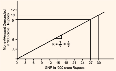
Figure 1 illustrates the demand for money. The horizontal axis shows GNP in thousand crore rupees and the vertical axis the amount of money demanded. The demand curve has a slope of k =  1/V = 1/3. If V = 3, then for an increase in GNP of Rs.27,000 crore, the amount of money demanded will be Rs.9,000 crore. If GNP increases to Rs.30,000 crore, the amount demanded will increase to Rs.10,000 crore. Thus, the amount of money demanded is directly related to the spending involved in GNP.

Figure 1: Demand for Money

Both the quantity theories considered V and k to be relatively stable. In their view V and k were determined by institutional considerations such as credit practices among various firms or between firms and households, and by technological factors such as the nature of communications which they felt will change slowly over time. As such they regarded V and k as relatively constant.

Constant k implies that the stock of money is the major determinant of aggregate demand. But, this assumption of constant k is an over simplification. Table below shows the behavior of V and k during the period 1982-2000.

Table 1
 The income velocity and the ratio of money supply to GNP

Q = Quick estimates

Source: Economic Survey 2000 - 01

Column 3 of the table shows the behavior of income velocity which is simply GNP/M and column 4 shows the behavior of k, which is nothing but M/GNP, or in other words 1/V. From the table it is clear that V and k are not constants through time and can indeed change substantially within a period of several years. However, the average arithmetic change in V is of the order of 0.2 per year, while no change exceeds 0.45. Though the number seems too small it is quite misleading to assume that k and V are relatively constant.

For example, let us consider a year in which Y = Rs.650 crore and M = Rs.130 crore and consequently V = 5 and k = 1/5. Now assume that the monetary authorities would like Y to grow by 5% i.e. they would like to have Y Rs.682.5 crore (i.e. 650 x 1.05) during the next year. What amount of money should they supply to have the desired level of Y. Obviously, it depends on their estimate of V or k. If V is expected to remain constant, the quantity of money to be supplied would appropriately be 1/5 x 682.05 = Rs.136.5 crore i.e. they would let M also increase by 5%. But, if the actual value of V turns out to be 5.2, the value of V that would result then would be Rs.709.8 crore. In other words, Y would grow at over 9.2 percent per year rather than the intended 5 percent. If the economy were already near full employment, it could produce a considerable amount of unwanted inflation. Thus, small fluctuations in V or k do have substantial repercussions on the level of economic activity.

We have seen that V and k are not constants but do fluctuate in the short run. The reasons for these fluctuations V and k are determined by the choices of the community and not by the monetary authority. Though stock of money is controlled by the monetary authority, the rate of expenditure relative to M is decided by the community. In terms of the k approach, people may choose to hold only small balances relative to their rate of expenditures, which will be reflected in a high rate of expenditures relative to the stock of money. On the other hand, if the people choose to hold larger balances relative to their expenditures, Y will be smaller relative to M. In terms of the velocity approach, people may choose to hold money balances longer before spending which will be reflected in a lower V while if they choose to hold money for a short span before spending, V will be high.

The choices of the community to hold or spend do not change in a haphazard manner but rather are systematically related to the state of economy. During periods of prosperity or boom velocity increases and during the periods of recession it declines or increases less rapidly. This is because during periods of prosperity, interest rates rise and an increase in interest rates encourages people to economize money holdings and to hold a larger fraction of its total assets in the form of earning assets. During periods of recession, interest rates tend to fall and people prefer to hold larger money balances.

A theory of demand for money should capture all these aspects. The quantity theory is, thus, not a satisfactory theory of the demand for money. To construct such a theory, interest rates should be introduced into the determination of demand for money.