Reference no: EM132814484

MAE306 Computer Aided Engineering - Nazarbayev University

Part A: Assume the function f(x) = sin(x)⋅e(-x/(20+c), x ∈ I = [0,100], with c being equal to the last digit of your student ID. Use MATLAB to compute the corresponding linear interpolant ^{^}f^(x) = ∑_i=0ⁿ f(x_i)Φ_i(x), xi , x ∈ ^~I and the L²-projection f¯(x) = ∑_i=0ⁿ ξ_iΦ_i(x), x ∈ I^~ for the following uniform mesh partitions: ^~I₁ = [0,10,20, ... ,100], ^~I₂ = [0,1,2, ... ,100], and ^~I₃ = [0,0.1,0.2, ... ,100].

For each case compute the corresponding norms, ||f(x) - f^(x)||²_L²(I), ||f(x) - f(¯ x)||_L²(I), and plot them in a single graph with respect to ^~I_i, i = 1,2,3. For the calculation of the involved integrals, you need to use either MATLAB's integral function or your own implementation of Simpson's rule with a minimum of (2n+1) quadrature points, where n is the number of subintervals in Ii; no other option is allowed.

Deliverables: MATLAB scripts and/or functions that implement the calculation of the approximant functions, the norm calculations, and the resulting graphs.

Report: Include in your report, at a minimum, 6 plots displaying f, f^ and f, f¯ for each mesh I_i, i = 1,2,3 along with the resulting L2-norm convergence graph with clear captions, legends and/or anno- tations, as required. Do not forget to include a table with the computed L2-norm values for all cases.

Part B: Assume that you would like to approximate the hyperbolic paraboloid (f(x, y) = xy) defined over the domain Ω shown below with C₁ and C₂ corresponding to the last and next to last digits of your student ID. For the approximation you will use the space of continuous piecewise linear func- tions and compute both the linear interpolant and L2-projection using triangulations, K_i, i = 1,2,3, with a maximum edge size of 0.5, 0.25 and 0.15 units, respectively. As in Part A, use MATLAB to compute the linear interpolant f^(x, y) = ∑ⁿ_i=1 f(pi)Φi(x, y), pi, x, y ∈ ^~K (Ω) and the L²-projection f¯(x, y) = ∑_i=1ⁿ ξiΦi(x, y), x, y ∈ K(Ω) for the 3 triangulations mentioned above. You will then compute the L²-norms, ||f(x, y) - f^(x, y)||²_L²(Ω), ||f(x, y) - f(¯ x, y)||²_L²(Ω), and plot them in a single graph with respect to K_i, i = 1,2,3. For the calculation of the involved integrals, you need to use either MATLAB's quad2d function or your own implementation of Simpson's rule for double integrals with a minimum of nt quadrature points in each direction, where nt is the number of triangles in ki; no other option is allowed.

Deliverables: MATLAB scripts and/or functions that imple- ment the calculation of the approximant functions, the norm calculations, and the resulting graphs.

Report: Include in your report, at a minimum, 6 surface plots displaying f, f^ and f, f¯ for each mesh ki, i = 1,2,3 along with the resulting L2-norm convergence graph with clear cap- tions, legends and/or annotations, as required. Do not forget to include a table with the computed L2-norm values for all cases.

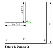
Figure 1: Domain Ω

Part C: Potential flow over symmetric airfoils

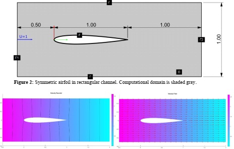
Develop a FEM solver that estimates the flow characteristics around symmetric 4 digit NACA foils of your choice with a zero angle of attack; generate three different NACA 4 digit symmetric airfoils using the tool provided while making sure that you use cosine spacing with closed TE and a minimum of 81 points for their representation. Consider an incompressible fluid and an irrotational velocity field which will allow your computational approach to be based on finding the unknown velocity potential Φ. Figure 2 shows the computational domain (Ω) and an example symmetric airfoil positioned with its leading edge at the coordinate system's origin. Assume a uniform velocity field with a speed parallel to x-axis with a magnitude of 1 speed unit (Γ1) and a velocity potential equal to 0 at Γ2. For all other boundaries (Γ) you should enforce a zero normal velocity component.

1. Develop the FEM computation approach required for computing the flow around the airfoils. All code parts must be developed by you without using any PDE toolbox functions except for the ones used for generating the domain mesh (triangulation) and plot functions that will allow the visualization of your results.

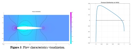
2. Develop the same computational method, as above, but this time use the functions provided by the PDE toolbox. Compare the results obtained here with the ones from step 1 by plotting and measuring differences for:
a. The velocity potential on Ω.
b. The velocity field on Ω.
c. The pressure distribution on Ω.
d. The pressure distribution on the airfoil.
See Figure 3 for examples of plot types you need to generate.

3. Compute the pressure distribution on the same airfoils using the xfoil BEM computational package; Save and compare your results with the pressure distributions obtained in steps 1&2. Make sure you use a pure potential flow solution from xfoil without taking into account viscosity.

4. Pick a non-symmetric NACA 4 digit airfoil or consider a non-symmetric flow for one of the previously computed symmetric airfoils. Compute the pressure distribution on the airfoil for this case and compare it against the corresponding one obtained from xfoil. As you might have guessed the results will not be in alignment. Explain why and attempt to modify your code to achieve results similar to the ones obtained from xfoil.