Reference no: EM131747086

1. Let X₁,. .., X_n be iid N(θ, θ²) where θ > 0 is an unknown parameter. Consider the following estimators of θ:
• The sample mean T₁(X₁,. .., X_n) = X¯
• The modified sample standard deviation

T₂(X₁,. .., X_n) = k_n S

where

S² = 1/n-1 ∑ⁿ_i=1 (X - X¯ )² and k_n = (√(n - 1) Γ(n-1/2))/(√2Γ(n/2)

and Γ is the Gamma function.
• The combined estimator

T₃ (X₁,. .., X_n) = (T₁(X₁,. .., X_n) + T₂(X₁,. .., X_n))/2

• The maximum likelihood estimator

T₄(X₁,. .., X_n) = √(X¯² + 4/n∑ⁿ_i=1 X_i² - X¯ )/2

• The sample mean absolute deviation

T₅ (X₁,. .., X_n) = 1/n∑ⁿ_i=1 |X_i - X¯|

• The sample median

T₆(X₁,. .., X_n) = inf{x ∈ R : F^(x) ≥ 0.5}
where F^(x) is the empirical cumulative distribution function (see Definitions 12 and 13 of the Lecture notes). In R you can compute this estimator by using quantile(x,probs=0.5,type=1)

1.1 Show that θ is scale parameter and then show that

Z_i = T_i/θ

is a pivot for all i ∈ {1, 2, 3, 4, 5, 6}.

1.2 Use the pivots Z₁,. .., Z₆ to construct 95% confidence intervals for θ and show the expressions for the endpoints of the six intervals as a function of T_i and the quantiles of the sampling distributions of Z_i when n = 30. To estimate those quantiles, you can use the Monte Carlo method with r = 10000.

1.3 Using n = 30 again, plot (in a single figure) the expected length of each of the confidence intervals as a function of θ in the interval (0, 5). Which interval is shortest on average for all values of θ ∈ (0, 5)? How does the combined estimator T₃ compared to T₁ and T₂ in terms of expected length? To estimate the expected lengths, you can use the Monte Carlo method with r = 10000.

1.4 For n = 30, plot (in a single figure) the mean square error (as a function of θ and in the interval (0, 5)) for all the six estimators.

2. Let X₁,. .., X_n be iid continuous random variables with density

f(x|µ, ∈) = (1 - ∈) Φ(x - µ) + ∈Φ (x - (µ + 10))
where Φ is the standard normal density. This density has the interpretation of being the mixture of two densities: one (say f₁(x|µ) = Φ(x - µ)) corresponding to a normal distribution with mean µ and variance one (with weight (1 - ∈)) and another density (say f₂(x µ) = Φ(x µ 10)) corresponding to a normal with mean µ+10 and variance equal to one (with weight ∈).

This family of densities is commonly used to model observations in the presence of outliers or aberrant observations. The idea is that we cannot observe directly form the first density f₁ which has mean µ and where µ is the actual parameter of interest. We can only observe samples which contain observations from f₁ but also some outlying observations we are not really interested in. These outlying observations follow a density with a notoriously diαerent mean which in this case is µ + 10. The weight ∈ is the average proportion of outlying observations in the sample. The main problem is that we cannot distinguish between an unusally large observation from f₁ from an outlying observation from f₂. They are all mixed-up and we need to decide what to do to minimize the influence of such outlying observations.

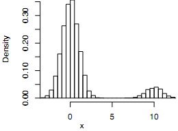
The following R function rand.f return random samples from the density f(x µ, ∈). To illustrate the shape of the densities, we have generated 10000 observations from f(x µ, ∈) with µ = 0 and ∈ = 0.1 and then plotted the corrresponding histogram. We can see that indeed there is a small proportion of the observations (10% on average) that have a mean 10 units larger than the mean of zero of the observations from f1. We need to modify our current known estimates of µ in order to deal with outliers and avoid bias. In Statistics, we say that we need a robust procedure.

rand.f<-function(n=10,mu=0,epsilon=0.1){
if (epsilon==0){
x<-rnorm(n,mean=mu,sd=1)
}else{
x<-rep(0,n)
for (i in 1:n){
u<-rbinom(1,size=1,prob=epsilon)
if (u==0){
x[i]<-rnorm(1,mean=mu,sd=1)
}else{
x[i]<-rnorm(1,mean=(mu+10),sd=sqrt(1))
}
}
}
return(x)
}
xx1<-rand.f(n=10000,mu=0,eps=0.1)
hist(xx1,50,freq=F,xlim=c(-3,12),xlab="x",main="f(x|0,0.1)")

f(x|0,0.1)

We consider the following three estimators of the parameter of interest µ.

The sample mean X¯ . This estimator of µ is biased upwards since the outlying observations are pulling the arithmetic mean above the target µ.
The sample median as defined in the previous question. This estimator is more robust than the mean to the presence of outliers since it does not take into account the magnitude of the outlying observations.

• The p% upper trimmed mean defined as:

µ˜_p =  (X₍₁₎ + X₍₂₎ + .. . + X_(N))/N

where X_(i) are the order statistics X₍₁₎ < X₍₂₎ < and N = ceiling((1-p) n). This estimator of µ removes the p% largest observations from the sample and then takes the arithmetic average of the remaining.

We want to test the hypotheses:

H₀ : µ = 0 vs H₁ : µ> 0

and we consider the following critical regions:

C₁ = {(x₁,. .., x_n) : x¯ > k₁} (1)
C₂ = {(x₁,. .., x_n) : median(x₁,. .., x_n) > k₂} (2)
C₃ = {(x₁,. .., x_n) : µ˜p > k₃} (3)

2.1 Using the Monte Carlo method with r = 10000, obtain the values of k₁, k₂ and k₃ to perform the tests at a significance level of α = 0.05 when n = 30, ∈ = 0.1. For C₃ you should use p = 0.3.

2.2 Plot the power functions (in a single figure) as a function of µ in the interval (0, 2). Explain the shape of all the three power functions. What happens when we decrease the value of p to p = 0.15 and if we increase to p = 0.5?

3. Let X be a continuous and positive random variable with probability density function g(x|θ) where θ > 0 is an unknown parameter. We do not know the functional form of g and the only thing we know about g is how to simulate random samples from g for given values of θ. We will use the R function rg for this purpose where the function can be downloaded as follows

The function rg has two arguments: n and theta which specify the sample size and the parameter value θ, respectively, and the function returns a generated random sample of size n. To simulate a random sample of size n = 5 from g(x|θ = 1) we can simply use

x.sample<-rg(n=5,theta=1)

x.sample
## [,1]
## [1,] 0.5718220
## [2,] 1.3856786
## [3,] 0.4198774
## [4,] 1.0478892
## [5,] 0.6905807

Suppose we are interested in the simple null hypothesis

H₀ : θ = θ₀

for some known θ₀ > 0 and that we are given a test statistic S in the form of an R function

The function S has two arguments: x and theta0 where x is a vector of observations and theta0 is the value of θ under the null hypothesis. For example, if we are interested in the simple null hypothesis

H₀ : θ = 1

and we have available the observed random sample x.sample generated above, then the value of the test statistic is given by

S(x=x.sample, theta0=1)

## [1] 0.2236653

Let X₁,. .., X_n be a random sample from the density g(x|θ) where the parameter θ > 0 is unknown. We want to test the hypotheses

H₀ : θ = 1 vs. H₁ : θ ≠ 1

3.1 How would you use the given test statistic S in order to construct a sensible critical region with a significance level α = 0.05 when n = 30. You must provide the specific form of the critical region as a subset of Rⁿ, in terms of the statistic S and not in terms of unspecified constants. You must use Monte Carlo with r = 10000.

3.2 Using n = 30 and the Monte Carlo method with r = 10000, plot the corresponding power function as function of θ in the interval θ ∈ (0, 2). Interpret the plot by answering questions like: Why is the power function large or small in diαerent regions of θ.

3.3 Plot histograms of samples of size n = 10000 for θ = 1, 5, 10, 15, 20. Also (in a diαerent figure) plot both the expected value and the variance of X under the density g as a function of θ in the interval (0, 6). How does θ changes the density of the observations?

3.4 Propose a new statistic T and show the corresponding critical region to test the hypotheses

H₀ : θ = 1 vs. H₁ : θ ≠ 1

with a significance level α = 0.05 when n = 30. You must provide the specific form of the critical region as a subset of R³⁰, in terms of the statistic T and not in terms of unspecified constants. You must use Monte Carlo with r = 10000. Plot the power of your proposed test in the interval θ ∈ (0, 2). How does the power of the test based on T compare to the one defined by S?

3.5 Given the data

x.sample<-c(1.373,2.29,1.434,0.747,1.45,1.912,0.405,0.607,0.515,0.548)

use the critical region based on your proposed statistic T to test the hypotheses

H₀ : θ = 1 vs. H₁ : θ ≠ 1
with a significance level of α = 0.1. What can you conclude?