Reference no: EM131374169

Question 1

Box office collection of 150 Bollywood movies were analysed using the variables described in Table 1.

Table 1. Data Dictionary

S.No	Variable	Variable Type	Code in SPSS output
1	Box office Collection (Y)	Numerical (in crores of rupees)	Box Office Collection
2	Release Time	Categorical with 4 levels	Releasing_Time_Festival Season Releasing_Time_Holiday Season Releasing_Time_Long Weekend Releasing_Time_Normal_Season
3	Genre	Categorical with 5 levels	Genre_Action (Action) Genre_Drama (Drama) Genre_Romance (Romance) Genre_Comedy (Comedy) Genre_Others (Other-G)
4	Movie Content	Categorical with 3 levels	Masala (Masala) Sequel (Sequel) Others (Other_C)
5	Director Category	Categorical with 3 levels	Director_A Director_B Director_O
6	Lead Actor Category	Categorical with 3 levels	Actor_A Actor_B Actor_O
7	Music Director Category	Categorical with 3 levels	Music_Dir_CAT A Music_Dir_CAT B Music_Dir_CAT C

8	Production House Category	Categorical with 3 levels	Prod_House_CAT A Prod_House_CAT B Prod_House_CAT C
9	Item Song	Binary variable	Item_Song (1 implies that the movie has an item song, 0 otherwise)
10	Budget	Numerical (in crores of rupees)	Budget
11	YouTube Views	Numerical	YouTube-V
12	YouTube Likes	Numerical	YouTube-L
13	YouTube Dislikes	Numerical	YouTube-D
14	Budget More than 35 crores	Categorical	Budget_35_Cr (1 if the budget is more than 35 crores 0 otherwise)

A simple linear regression model was developed between Box office collection and budget. SPSS output of the model is shown in Tables 2-3 and Figures 1-2.

Model 1

Y (Box Office Collection) = β₀ + β₁x Budget

Table 2. Model Summary

Model	R	R Square	Adjusted R Square	Std. Error of the Estimate
1	.650a			72.02261

a. Predictors: (Constant), Budget
b. Dependent Variable: Box_Office_Collection

Table 3. Coefficientsa

Model	Unstandardized Coefficients		Standardized Coefficients	T	Sig.
	B	Std. Error	Beta
(Constant)	-8.354	8.535	.650	-.979	.329
1
Budget	2.175	.210		10.381	.000

a. Dependent Variable: Box_Office_Collection

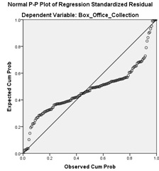
Figure 1. Normal P_P plot for Model 1

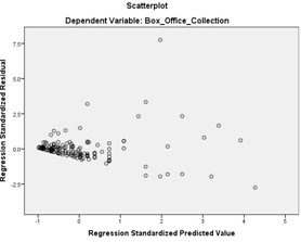
Figure 2. Residual plot for Model 1

Question 1.1

Which of the following statements are correct (more than one may be correct)? Tick (?) all right answers or highlight the correct statements with color.

1. The model explains 42.25% of variation in box office collection.
2. There are outliers in the model.
3. The residuals do not follow a normal distribution.
4. The model cannot be used since R-square is low.
5. Box office collection increases as the budget increases.

Question 1.2

Mr Chellappa, CEO of Oho Productions (OP) claims that the regression model in Table 3 is incorrect since it has negative constant value. Comment whether Mr Chellappa is correct in his assessment about the model.

A second model is developed between ln(Box office collection) and movie release time:

Model 2

ln(Y) = β₀ + β₁ x Release Time FestivalSeason + β₂ x Release Time Long Weekend + β₃ x Release Time Normal Season + ε

The regression output for Model 2 is given in Table 4.

Table 4 Coefficients

Model	Unstandardized Coefficients		Standardized Coefficients	t	Sig.
	B	Std. Error	Beta
(Constant)	2.685	.396		6.776	.000
Releasing_Time_Festival_Season	.727	.568	.136	1.278	.203
Releasing_Time Long_Weekend	1.247	.588	.221	2.122	.036
Releasing_Time Normal_Season	.147	.431	.041	.340	.734

a. Dependent Variable: Ln(Box Office Collection)

Question 1.3

What is the average difference in the box office collection when a movie is released during a holiday season (Releasing_Time_holiday_season) versus movies released during normal season (Releasing_Time_Normal_Season)? Use a significance value of 5%.

Question 1.4

Mr Chellappa of Oho productions claims that the movies released during long weekend (Releasing_Time_Long_Weekend) earn at least 5 crores more than the movies released during normal season (Releasing_Time_Normal_Season). Check whether this claim is true (use α = 0.05).

A stepwise regression model is developed between ln(Box Office Collection) and all the predictor variables listed in Table 1. The outputs are shown in Tables 5-6.

Table 5 Model Summary

Model	R	R Square	Adjusted R Square	Std. Error of the Estimate
1	.709a	.503	.499	1.20651
2	.763b	.581	.576	1.11050
3	.787c	.620	.612	1.06210
4	.802d	.643	.633	1.03307
5	.810e			1.01749
6

Table 6. Coefficients in the model (in the order in which it was added to the model)

Model		Unstandardized Coefficients		Standardized Coefficients	T	Correlations
		B	Std. Error	Beta		Zero-order (direct)	Partial	Part
	(Constant)	3.573	.249		14.346
	Budget_35_Cr	1.523	.207	.443	7.342	.709	.525	.356
	Youtube_Views	1.1710-07	.000	.242	4.426	.538	.348	.214
Step 6	Prod_House_CAT A	.562	.185	.165	3.033	.444	.247	.147
	Music_Dir_CAT C	-.645	.199	-.177	-3.245	-.483	-.263	-.157
	GenreComedy	.456	.197	.115	2.312	.006	.190	.112
	Director_CAT C	-.434	.203	-.123	-2.143	-.509	-.177	-.104

Question 1.5

What is the variation in response variable, ln(Box office collection), explained by the model after adding all 6 variables?

Question 1.6

Which factor has the maximum impact on the box office collection of a movie? What will be your recommendation to a production house based on the variable that has maximum impact on the box office collection?

Question 1.7

Compare the regressions in Model 2 (Table 4) and Model 3 (Tables 5 and 6). None of the variables in Model 2 are statistically significant in Model 3. Can we conclude that the variables in Model 2 have no association relationship with Box Office Collection? Explain clearly.

Question 1.8

Among the variables in Table 6, which variable is not useful for practical application of the model? Clearly state your reasons.

Question 2

The yearly US Sales of domestically produced cars is collected for the period 1970-1999, along with the data on the following:
PriceIndex - CPI for Transportation
Income - Total Disposable Income in the US (billions of dollars) Interest - Prime Interest Rate (%) Charged by Banks

	Year	Sales	PriceIndex	Income	Interest
Year	1
Sales	-0.5453	1.0000
PriceIndex		-0.6089	1.0000
Income		-0.5033		1.0000
Interest		-0.3842			1.0000

SPSS was used to carry out Stepwise Regression in order to predict Sales. The summary of the models fitted in the first 2 steps; the ANOVA table and Coefficients table obtained are given below.

Model Summary

Model	R	R Square	Adjusted R Square	Std. Error of the Estimate
1
2	.708b	.502	.465	760459.004

a. Predictors: (Constant),
b. Predictors: (Constant), , Interest
c. Dependent Variable: Sales

ANOVA

Model		Sum of Squares	df	Mean Square	F	Sig.
1	Regression
	Residual
	Total
2	Regression	1.571E13				.000b
	Residual	1.561E13
	Total	3.132E13

Coefficients

Model		Unstandardized Coefficients		Standardized Coefficients	t	Sig.
		B	Std. Error	Beta
1	(Constant)	9102897.600	433224.149	-.609	21.012	.000
		-17258.553	4248.694		-4.062	.000
2	(Constant)	1.023E7	576427.867		17.740	.000
		-16873.654	3853.737	-.595	-4.379	.000
	Interest	-124592.212	46820.081	-.362	-2.661	.013

a. Dependent Variable: Sales

Question 2.1

a) What is the predictor variable used in Model 1? Explain clearly.
b) What proportion of variation in Sales does this predictor variable explain in model 1? Explain clearly.
c) What is the Std. Error of the Estimate for Model 1? Explain clearly.

Question 2.2

a) What is the magnitude of the semipartial (or part) correlation for the variable ‘Interest' in Model 2? Explain.
b) Carry out an appropriate test, at 95% confidence level, to determine if Model 2 as a whole is valid (significant). State the null and alternate hypotheses and show all work.
c) Given no change in the other significant explanatory variables, can it be concluded from Model 2 that ‘Interest' has a higher impact on ‘Sales' than the other variable used in the model. Explain clearly.

Question 2.3: Can it be concluded, at 95% confidence level, that an increase in ‘Interest' rate by 5% decreases yearly Sales by at least 250000 units or more? Show all work.

Question 2.4: What can you say about the relationship between ‘Interest' and the other predictor variable used in Models 1 and 2? Explain clearly.

Question 2.5: The partial correlation of the excluded variables; after Model 2 was fitted; are 0.184 and Conduct an appropriate test, at 95% confidence level, to determine if one of these excluded variables should be added to the regression model. State the null and alternate hypotheses and show all work.

Question 3:

A large grocery store in the US wishes to understand the key drivers that determine the amount spent per transaction by their customers. Therefore, it obtained a random sample of 4000 transactions with information on the amount spent (Revenue), the product category on which the transaction was made (Product Family), the annual income of the customer (Annual income), the number of children in the household the customer belongs to, and finally whether the customer owns a home or not. A ‘snapshot' of part of the data is provided below.

Homeowner	Children	Annual Income	Product Family	Revenue
Y	2	$30K - $50K	Food	$27.38
Y	5	$70K - $90K	Food	$14.90
N	2	$50K - $70K	Food	$5.52
Y	3	$30K - $50K	Food	$4.44
Y	3	$130K - $150K	Drink	$14.00
Y	3	$10K - $30K	Food	$4.37
Y	2	$30K - $50K	Food	$13.78
Y	2	$150K +	Food	$7.34
Y	3	$10K - $30K	Non-Consumable	$2.41
N	1	$50K - $70K	Non-Consumable	$8.96
N	0	$30K - $50K	Food	$11.82

In order to enable regression analysis, the following indicator (dummy) variables were created: Own_Hm = 1 (Yes to Homeowner), 0 otherwise,

Ann_Inc2 = 1 (Annual Income in the range $30K - $50K), 0 otherwise Ann_Inc3 = 1 (Annual Income in the range $50K - $70K), 0 otherwise

Ann_Inc4 = 1 (Annual Income in the range $70K - $90K), 0 otherwise

Ann_Inc5 = 1 (Annual Income in the range $90K and above), 0 otherwise Prod_Fam2 = 1 (Product Family is Drink), 0 otherwise

Prod_Fam3 = 1 (Product Family is Non-Consumable), 0 otherwise.

The following outputs were generated using this data

Regression Output 1 (Revenue($) Response Var)

Regression Statistics

Multiple R	0.0340
R Square	0.0012
Adjusted R Square	0.0002
Standard Error	8.1499
Observations	4000.0000

ANOVA

	df	SS	MS	F	Significance F
Regression	4.0000	306.4494	76.6123	1.1535	0.3294
Residual	3995.0000	265348.3672	66.4201
Total	3999.0000	265654.8166
	Coefficients	Standard Error	t Stat	P-value
Intercept	12.6841	0.2786	45.5352	0.0000
Ann_Inc2	0.2787	0.3588	0.7766	0.4374
Ann_Inc3	0.7617	0.4106	1.8551	0.0637
Ann_Inc4	0.4524	0.4712	0.9602	0.3370
Ann_Inc5	-0.0130	0.4229	-0.0307	0.9755

Regression Output 2 (Revenue($) Response Var) 

Regression Statistics
Multiple R	0.059
R Square	0.004
Adjusted R Square	0.003
Standard Error	8.137
Observations	4000.000

ANOVA
	df	SS	MS	F	Significance F
Regression	1.000	933.834	933.834	14.103	0.000
Residual	3998.000	264720.983	66.213
Total	3999.000	265654.817
	Coefficients	Standard Error	t Stat	P-value
Intercept	12.136	0.255	47.564	0.000
Children	0.326	0.087	3.755	0.000

 Regression Output 3(Revenue($) Response Var)

 

Regression Statistics
Multiple R	0.046
R Square	0.002
Adjusted R Square	0.002
Standard Error	8.144
Observations	4000.000
ANOVA
	df	SS	MS	F	Significance F
Regression	2.000	550.538	275.269	4.150	0.016
Residual	3997.000	265104.278	66.326
Total	3999.000	265654.817
	Coefficients	Standard Error	t Stat	P-value
Intercept	13.192	0.152	86.958	0.000
Prod_Fam2	-0.975	0.458	-2.131	0.033
Prod_Fam3	-0.743	0.332	-2.240	0.025

 Regression Output 4 (Revenue($) Response Var)

Regression Statistics
Multiple R	0.075
R Square	0.006
Adjusted R Square	0.005
Standard Error	8.131
Observations	4000.000

ANOVA

	df	SS	MS	F	Significance F
Regression	3	1496.798	498.933	7.548	0
Residual	3996	264158.02	66.106
Total	3999	265654.82
	Coefficients	Standard Error	t Stat	P-value
Intercept	12.361	0.267	46.345	0
Children	0.329	0.087	3.783	0
Prod_Fam2	-0.992	0.457	-2.171	0.03
Prod_Fam3	-0.747	0.331	-2.256	0.024

Regression Output 5 (Revenue($) Response Var) Child_Fam3 = Children*Prod_Fam3

Regression Statistics

Multiple R	0.080
R Square	0.006
Adjusted R Square	0.006
Standard Error	8.127
Observations	4000.000

ANOVA

	df	SS	MS	F	Sig F
Regression	3.000	1708.947	569.649	8.624	0.000
Residual	3996.000	263945.870	66.053
Total	3999.000	265654.817
	Coefficients	Standard Error	t Stat	P-value
Intercept	12.214	0.258	47.399	0.000
Children	0.393	0.090	4.379	0.000
Prod_Fam2	-1.010	0.455	-2.218	0.027
Child_Fam3	-0.322	0.112	-2.882	0.004

Use the information given above to answer the following questions.

For each question give adequate explanation and support your answer with given information precisely. Wherever required assume α = 0.05 for significance level.

a) Rank the income groups based on average revenue obtained per transaction in the sample data from largest to smallest. Provide precise reasons as to how you obtained this ranking. Is this ranking valid for the population? What is the average revenue per transaction obtained for the income group ($10K-$30K)?

b) The grocery store wishes to estimate the average amount spent per transaction on non- consumables. Provide the most accurate estimate possible. Provide details on how you obtained this estimate.

c) If in regression output 3, if the base chosen in product family is drinks (Prod_Fam2), then what will be the corresponding prediction equation?

d) Is there a significant difference in the average amount spent per transaction between that on drinks and non-consumables? Why or Why not? Provide precise reasons.

e) The grocery store wishes to target those customers, as well as items on which the amount spent is maximum. Assuming that no customer has more than five children, identify the appropriate customer segment as well as the appropriate product family. Provide precise reasons behind your answer.

f) What is the chance that a customer with 3 children will spend more than $10.00 on food items per transaction? Provide details on your calculations.

g) Do the number of children effect food purchases more than non-consumables? Why or why not? State your reasons precisely. (3 points)
h) If the grocery store has reason to believe that in addition to the independent variables considered in Regression Output 4, homeowners spend significantly more on non-consumables than non- home owners on any product category. If so, how will you modify the model provided in Regression Output 4? Provide the model in β terms. If you are adding new variables to the model, provide details on what you expect the β value to be. Positive? Negative?

Question 4

Go through the case, "Oakland A" and the spreadsheet supplement (Ref: Moodle/Cases and Materials/Module 3). Does mark Nobel increase attendance? If so, how much is the increase worth for Oakland? Support your decision through an appropriate regression model.

Question 5

Box office success of Bollywood movies was analysed using the following variables using logistic regression model. The data model is provided in the following table.

Sl. No	Variable	Variable Type	Code in SPSS output
1	Box office success (Y)	Categorical	1 = Success 0 = Failure
2	Release Data	Categorical     with                      4 levels	1 = Festival Season (FS) 2 = Holiday Season (HS)

			3 = Long Weekend (LW) 4 = Other Season (OS)
3	Genre	Categorical     with                      5 levels	1 = Action (Action) 2 = Drama (Drama) 3 = Romance (Romance) 4 = Comedy (Comedy) 5 = Others (Other-G)
4	Movie Content	Categorical     with                      3 levels	Masala (Masala) Sequel (Sequel) Others (Other_C)
5	Director Category	Categorical     with                      3 levels	Director_A Director_B Director_O
6	Lead Actor Category	Categorical     with                      3 levels	Actor_A Actor_B Actor_O
7	Item Song	Binary variable	1 (Movie has an item song) 0 (otherwise)
8	Budget	Numerical (in crores of rupees)	Budget
9	YouTube Views	Numerical	YouTube-V
10	YouTube Likes	Numerical	YouTube-L
11	YouTube Dislikes	Numerical	YouTube-D

A logistic regression model was developed using Budget as independent variable and box office success as the dependent variable (ln(Π/(1-Π) = β₀ + β₁ x Budget.

The SPSS model-output is shown below (Tables 1-3)

Table 1 Omnibus Tests of Model Coefficients

		Chi-square	df	Sig.
	Step	4.000	1	.046
Step 1	Block	4.000	1	.046
	Model	4.000	1	.046

Table 2 Classification Table

	Observed	Predicted
		Success   Failure		Percentage Correct
		0	1
	0	2	17	10.5
	SuccessFaliure
Step 1	1	3	41	93.2
	Overall Percentage			68.3

a. The cut value is .500

Table 3 Variables in the Equation

		B	S.E.	Wald	df	Sig.	Exp(B)
Step 1a	Budget	-.016	.008	3.825	1	.050	.984
	Constant	1.621	.503	10.395	1	.001	5.058

a. Variable(s) entered on step 1: Budget.

Question 5.1

Calculate the budget for which the box office success and failure are equally likely.

Question 5.2

Is there a sufficient evidence to conclude that the higher budget movies are more likely to fail at the box- office?

Question 5.3

A production house is making a movie with 100 crore budget; what is the success probability for this movie?

Question 5.4

Calculate the optimal cut-off probability when the cost of classifying failure at box office (0) as success at the box office (1) is five times costlier than the cost of classifying success (1) as failure (0). Show all calculations.

Step number: 1

			Observed	Groups	and	Predicted	Probabilities
	8	+																	+
		I																	I
		I													1				I
F		I													1				I
R	6	+													1		1	1	+
E		I													1		1	1	I
Q		I													1	1	1	1	I
U		I													1	1	1	1	I
E	4	+													0	0	11	111	+
N		I													0	0	11	111	I
C		I							1						0	0	11	1111	I
Y		I							1						0	0	11	1111	I
2		+							1	1	1	1		1	0	0	001111111		+
		I							1	1	1	1		1	0	0	001111111		I
		I	0  1					1 0 1	0	0	0	0	1	1	0	10	000111111		I
		I	0  1					1 0 1	0	0	0	0	1	1	0	10	000111111		I

Predicted ---------+---------+---------+---------+---------+---------+-------+---------+---------+---------- Prob:        0         .1        .2        .3      .4        .5      .6        .7        .8        .9        1

Group:        00000000000000000000000000000000000000000000000000111111111111111111111111111111111111111111111111

Predicted Probability is of Membership for 1 The Cut Value is .50

Symbols: 0 - 0; 1 - 1; Each Symbol Represents .5 Cases.

Figure 1. Classification plot for model 1

A second model is developed using the variable, "item song", the SPSS output is shown in tables 4-5.

Table 4 Classification Table

	Observed	Predicted
		SuccessFaliure		Percentage Correct
		0	1
	0	11	8	57.9
	SuccessFaliure
Step 1	1	20	24	54.5
	Overall Percentage			55.6

a. The cut value is .700

Table 5 Variables in the Equation

		B	S.E.	Wald	df	Sig.	Exp(B)
Step 1a	ItemSong	-.501	.202	6.151	1	.013	.606
	Constant	1.099	.408	7.242	1	.007	3.000

a. Variable(s) entered on step 1: ItemSong.

Question 5.5

Calculate the difference in success probabilities for movies with item song and movies without item song.

Question 5.6

Which is a better model (budget as an independent variable vs item song as an independent variable). Clearly state your reasons.

A stepwise logistic regression model is shown in tables 6 and 7 using significance α = 0.10. 35_Cr_Budget is a derived variable which takes value 1 if the movie budget is more than 35 crores and 0 otherwise.

Table 6 Classification Table

	Observed		Predicted
			SuccessFaliure		Percentage Correct
			0	1
Step 1	SuccessFaliure	0	14	5	73.7
		1	17	27	61.4
	Overall Percentage				65.1
Step 2	SuccessFaliure	0	14	5	73.7
		1	10	34	77.3
	Overall Percentage				76.2
Step 3	SuccessFaliure	0	12	7	63.2
		1	9	35	79.5
	Overall Percentage				74.6

Step 4	SuccessFaliure	0	13	6	68.4
		1	9	35	79.5
	Overall Percentage				76.2
Step 5	SuccessFaliure	0	15	4	78.9
		1	9	35	79.5
	Overall Percentage				79.4
Step 6	SuccessFaliure	0	13	6	68.4
		1	10	34	77.3
	Overall Percentage				74.6

a. The cut value is .700

Table 7 Variables in the Equation

		B	S.E.	Wald	df	Sig.	Exp(B)
Step 1a	35_Cr_Budget	-1.492	.606	6.063	1	.014	.225
	Constant	1.686	.487	11.998	1	.001	5.400
	YoutubeL	.000	.000	4.294	1	.038	1.000
Step 2b	35_Cr_Budget	-2.227	.694	10.285	1	.001	.108
	Constant	1.108	.550	4.055	1	.044	3.028
	Budget	-.027	.017	2.356	1	.125	.974
Step 3c	YoutubeL	.000	.000	5.903	1	.015	1.000
	35_Cr_Budget	-1.243	.911	1.860	1	.173	.289
	Constant	1.596	.624	6.554	1	.010	4.935
	Budget	-.034	.020	2.877	1	.090	.967
	YoutubeL	.000	.000	6.858	1	.009	1.000
Step 4d	DirectorA	1.544	.890	3.008	1	.083	4.683
	35_Cr_Budget	-1.621	.981	2.730	1	.098	.198
	Constant	1.556	.650	5.733	1	.017	4.742
	Budget	-.032	.021	2.393	1	.122	.969
	YoutubeL	.000	.000	7.067	1	.008	1.000
Step 5e	DirectorA	1.669	.902	3.427	1	.064	5.308
	ActorA	-1.327	.934	2.019	1	.155	.265
	35_Cr_Budget	-1.046	1.038	1.015	1	.314	.351
	Constant	1.972	.774	6.492	1	.011	7.187
	Budget	-.043	.018	5.579	1	.018	.958
	YoutubeL	.000	.000	7.370	1	.007	1.000
Step 6e	DirectorA	1.602	.895	3.206	1	.073	4.961
	ActorA	-1.622	.862	3.543	1	.060	.197
	Constant	2.132	.745	8.177	1	.004	8.429

a. Variable(s) entered on step 1: lt_35_Cr_Budget.

b. Variable(s) entered on step 2: YoutubeL.

c. Variable(s) entered on step 3: Budget.

d. Variable(s) entered on step 4: DirectorA.

e. Variable(s) entered on step 5: ActorA.

Question 5.7

Consider all the information in tables 1 to 7, which model you would recommend to predict the movie success at the box office? Clearly state your reasons.

Question 6

Read the case,"Breaking Barriers - Micro-mortgage analytics". Using the data provided, develop a credit rating model that Shubham can use. (Ref: Moodle/Cases and Materials/Module 3)

Question 7

A Micro-Mortgage company classifies customers into three categories (1, 2 and 3). Category 1 applicants are denied loan, Category 2 applicants are charged an interest rate of 14% per annum and Category 3 applicants are charged an interest rate of 18%. The variables considered in the model are shown below:

Sl. No	Variable	Variable Type	Code in SPSS output
1	Customer Classification	Categorical                          (3 levels)	1    = Category 1 2    = Category 2 3    = Category 3
2	Disposable Income	Numerical	DI
3	Loan to Value ratio	Numerical	LTV
4	Instalment to Income Ratio	Numerical	IIR
5	Marital Status	Categorical	MS = 1 = Married MS = 0 = Unmarried
6	Age	Numerical	Age
7	Old Emi	Categorical	Old Emi = 1 applicant with old EMI   Old emi = 0 otherwise

SPSS regression output using category 3 as base category is provided below:

Match_Oa		B	Standar d Error	Wald	Sig.	Exp(B)
1	Intercept	1.720	0.850	4.095	0.043	5.585
	DI	-0.120	0.050	5.760	0.016	0.887
	LTV	-0.521	0.260	4.015	0.045	0.594
	IIR	-0.220	0.100	4.840	0.028	0.803
	MS	0.850	0.620	1.880	0.170	2.340
	AGE	-0.340	0.240	2.007	0.157	0.712
	OLD EMI	-1.120	0.390	8.247	0.004	0.326
2	Intercept	0.650	0.280	5.389	0.020	1.916
	DI	-0.580	0.270	4.615	0.032	0.560
	LTV	0.960	0.850	1.276	0.259	2.612
	IIR	0.540	0.320	2.848	0.092	1.716
	MS	0.710	0.330	4.629	0.031	2.034
	AGE	-0.220	0.150	2.151	0.142	0.803
	OLD EMI	0.150	0.850	0.031	0.860	1.162

The reference category is 3.

Question 7.1
Comment whether the marital status has any statistical significance on the probability of loan denial. Clearly state your reasons.

Question 7.2
What percentage of the applicants with a DI=20, LTV = 0.5, IIR = 0.8, MS = 0 and Old EMI = 0 will be given a loan at 18% interest? Use only statistically significant variables and assume that the changes in the coefficient values are negligible due to dropping of insignificant variables.

Question 8
Read the case, "Fraud analytics at MCA technology solutions - Predicting Earnings Manipulation by Indian Firms". Develop a model using logistic regression and Random Forest to predict fraudulent transactions. (Ref: Moodle/Cases and Materials/Module 3)