Reference no: EM132384906

Experiment : Modeling the Industrial Plant Emulator

Objectives

1. To understand how to model rotational motion systems

2. To learn how to experimentally determine the physical parameters of the system

3. To use the experimental results in future feedback control experiments

Theory

General Model

The industrial plant emulator is a rotational motion system. From Newton's Law
Jα = ΣΤ

J = inertia
α = angular acceleration
Τ = torque

Torques can include an applied torque from the servomotor and opposing torques due to friction effects and torsion. A general differential equation model of the system is given by

Jd²θ/dt²+ c dθ/dt + Kθ = Τd

J = inertia (Kg - m²)
c = viscous friction (N-m/(rad/sec))
K = torsion constant (N-m/rad)
Τd = applied torque (N-m)
θ = angular position (rad)

In this experiment, torsion will not be a factor. The transfer function (setting K = 0) is given by

θ(s)/ Τ(s)= 1 +(Js²+ cs)

Speed Reduction Assembly

The industrial plant emulator has a speed reduction assembly (pulleys and belts) to control the speed of the load disc relative to the drive disc. The diagram below illustrates the system. Fixed pulleys at the drive and inertia discs have 12 teeth and 72 teeth respectively. Four pulleys are available for the SR Assembly: 18 teeth, 24 teeth, 36 teeth, and 72 teeth. All possible combinations, along with the resulting speed reduction are shown on the last page of this lab.

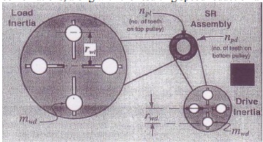
In our transfer function model, if θ(t) is the position of the drive disc and Τ is the applied torque by the drive motor, then J must be the total inertia seen at the drive disc and c must be the total viscous friction seen at the drive disc. The total inertia seen at the drive disc is given by

Jd* = Jdd + Jwd + Jp(12/n_pd)²+ (Jld + Jwl)(n_pl/72)² (12/n_pd) ²

Jd* = Total inertia reflected to the drive disc
Jdd = Inertia of the drive disc plus the drive motor, encoder, drive/disc motor belt and pulleys
Jwd = Inertia of any weights placed on the drive disc
Jp = Inertia of the pulleys in the SR assembly
Jld = Inertia of the load disc plus the disturbance motor, encoder, Load/disc motor belt and pulleys
Jwl = inertia of any weights place on the load disc

The same formula applies to viscous friction by replacing all J's with associated c's.

It is also important to be able to relate the speed of the load disc to the speed of the drive disc and the torque applied to the drive disc to the effective torque applied at the load disc. The following relationships hold:

_{Speed of Load Disc}dθ_l /dt = (n_pl/72)(12/n_pd) dθd/dt _{Speed of Drive Disc}

_{Torque at Load Disc}Τ_l= (72/npl)(npd/12) Τ_{d  Torque applied to Drive Disc}
 
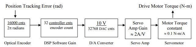
Hardware Gain

The hardware gain for the system is given by:

K_HW = K_sK_cK_aK_tK_e            N-m/rad

K_s = Software Gain = 32 controller input counts/encoder or ref input counts

K_c = DAC Gain = 10V/32,768 DAC counts

K_a = Servo Amp Gain ≈ 2 amps/volt

K_t = Servo Motor Torque constant ≈ 0.1 N-m/amp

K_e = Encoder gain = 16,000 pulses/ 2Π radians

The hardware gain simply translates a tracking error in a control torque for the drive motor.

Procedure

Part I: Determining the Hardware Gain, K_HW

The formula for hardware gain discussing in the theory section indicated two quantities, servo amp gain and servo motor torque constant that were only known approximately. The following procedure will provide a better estimate of the hardware gain.

1. Turn off the power to the Controller Box. Loosen the SR assembly clamp so that the belt can be removed from the drive disc. (It is not necessary to take the entire assembly apart, simply make sure the drive belt will not interfere with the motion of the drive disc)

2. Add four 500g brass weights to the drive disc. The weights must be evenly distributed on the drive disc. Align the edge of the weights to the edge of the drive disc. Since the drive disc has a diameter of 13.21 cm and the brass weights have a diameter of 4.95 cm, the distance from the center of the weights to the shaft center-line is given by

Dist to Shaft = 13.21/2 - 4.95/2 = ________ cm = _________ m

3. Replace the plexiglass safety cover and turn on the Controller Box.

4. Calculate the total inertia at the drive disc as follows:

First calculate the mass of the drive disc given that the diameter of the drive disc is 13.21 cm, the thickness is 0.47 cm and the density is 2.71 g/cm³.

Mass Drive Disc = ________ g = _________ Kg

Next calculate inertia of the drive disc using the formula

Jdisc = (Mass of Drive Disc)*(Diameter of Drive Disc in m)² / 8 = ___________ Kg-m²

Next calculate the inertia of the 4 weights using the formula

Jwd = 4*0.5Kg*(0.0413m)² + 4*0.5Kg*(Diameter of Weights in m)² /8 = _______ Kg-m²

From manufacturer's specifications, the drive motor inertia is Jmotor = 3.8*10-5 Kg-m²

Neglecting inertia of the encoder and the belt and pulleys between the motor and the drive disc, calculate the total inertia at the drive disc

Jd = Jdisc + Jmotor + Jwd = __________ Kg-m²

5. Make sure the user units in the Set-up menu of the ECP program are in counts.

6. Under the Set-up menu, select Control Algorithm and set Ts = 0.002652 s.

7. Next go to Trajectory under Command and select Step, Set-up. Choose an Open Loop Step then set the step size to 2.0 volts, duration to 200 ms with 1 repetition.

8. Under the Data menu, choose Set up Data Acquisition and select Encoder #1 only and specify data sampling every 5 (five) servo cycles.

9. Under Utility, select Zero Position, to zero the Encoder Position.

10. The system is now set up to accelerate the drive disc with a 2.0V input to the servo amp for 200 ms while acquiring data every 13 ms. In the Command menu, select Execute then Run. You should see the drive disc accelerate for 200 ms then decelerate.

11. In the Plotting menu, select Set-up Plot and choose Encoder #1 Velocity. Then select Plot Data. You should see a plot similar to the one shown below. The slope (i.e., derivative) of the curve will give acceleration. Label appropriate points on the plot below and calculate the positive slope to get acceleration in counts/s².

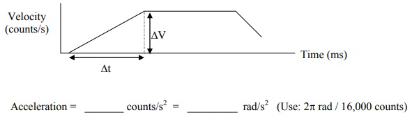
12. Go back to Set-Up plot and select Encoder #1 Acceleration instead of Velocity. The acceleration is numerically derived by taking two derivatives of the actual position data. What do you notice about the acceleration plot?

13. If we assume negligible friction, then Jα = Τ. Using the inertia determined in Step 4 and the acceleration determined in Step 10, calculate the applied drive torque, Τ.

Τ = Jα = _________ N-m

Now calculate the product of the Servo Amp Gain and the Servo Motor Torque constant using the relationship

KaKt(Applied Open-LoopVoltage) = Τ

KaKt = ___________ N-m/V

Finally, calculate the hardware gain, KHW

KHW = KsKcKaKtKe = _______________ N-m/rad

Ks = Software Gain = 32 controller input counts/encoder or ref input counts

Kc = DAC Gain = 10V/32,768 DAC counts

Ke = Encoder gain = 16,000 pulses/ 2Π radians

Part II: Measuring the Inertia at the Drive Disc

1. Turn off the power to the Controller Box. Remove the plexiglass cover and remove the brass weights from the drive disc. Put the safety cover back on.

2. Turn the power on to the Controller Box.

3. Under the Set-up menu, choose Control Algorithm. Use the following settings:

Ts = 0.002652 sec

Continuous Time Control. Select

PI with Velocity Feedback (Kp = 0.5, Kd = 0.001, Ki=0)

Implement the Controller.

4. Gently touch the drive disc with a non-sharp object to verify that the controller is implemented and is stable.

5. Enter the Command menu, go to trajectory, and select Step, Set-up. Choose a closedloop step with a step size of 1000 counts, a duration of 1000 ms and 1 repetition.

6. Under the Data menu, select Encoder #1 and Commanded Position as data to acquire and specify data sampling every 1 servo cycle. (Every 2.652 ms)

7. Under the Utility menu, select Zero Position to zero the encoder positions.

8. Select Execute from the Command menu then select Run.

9. Under the Plotting menu, choose Encoder #1 Position and Commanded Position then select Plot Data. You should see a decaying oscillating response similar to the one shown below

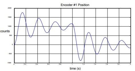
10. From the plot, estimate the natural frequency as follows:

ω_n ≈ number of cycles,n = _________ Hz = _________ rad/s time for n cycles

Use 1 or 2 cycles early in the plot since later cycles are dominated by nonlinear friction effects. You can zoom in by using Axis Scaling under Plotting. Label the plot above with the data points you used to determine natural frequency.

11. From the plot, estimate the damping, ?, as follows

ζ ≈ 1/(2Πn)*ln (Xi/Xf) = _____________________

Xi = output amplitude at first peak

Xf = output amplitude at a peak n cycles later

The closed-loop control system that was just implemented is modeled in the block diagram below.

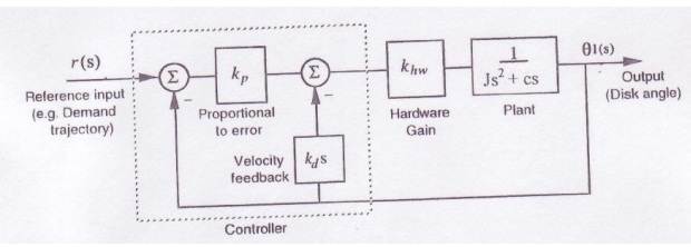
It can be shown that the closed-loop transfer function is given by

θ(s)/ R(s)= (K_pK_HW/J)/ (s² + [(c + K_HWKd)/J]s + K_pK_HW/J )= ω_n²/( s² + 2ζω_ns + ω_n²).

Equating coefficients in the denominator and doing a little algebra yields the following:

ω_n = √ KpKHW/J

ζ = (1/2ω_n)(c + K_HWKd)/J7

12. Using the equation above for ω_n, the proportional gain Kp = 0.5 implemented in the experiment, and the hardware gain K_HW calculated in Part A, calculate the inertia of the drive disc, Jdd.

Jdd = _________ Kg-m²

How does your experimental Jdd compare to the calculated Jd in Part A #4? Remember to subtract off the weights from your answer in Part A #4 since they were not used in this procedure.

Part III: Measuring the Inertia of the Load Disc

1. Turn off the Controller Box. Remove the plexiglass safety cover and set up the system in Test Case #4 (See last page of this lab). Put the safety cover back on.

2. Repeat Steps 2-11 from Part B. Roughly sketch your Encoder #1 Position plot below labeling key points used for calculating ?n and ?.
ω_n ≈ (number of cycles,n / time for n cycles)= _________ Hz = _________ rad/s

ζ ≈ 1/(2Πn) * ln (Xi/Xf) = _____________________

Xi = output amplitude at first peak

Xf = output amplitude at a peak n cycles later

3. Determine Jd* (total inertia seen at the drive) using the relationship

ω_n = √ KpK_HW/Jd*, the measured ω_n determined above, Kp = 0.5, and the measured KHW from Part A.

Jd* = ____________ Kg-m²

4. Now calculate the inertia of the load disc, Jld using the following formula and the manufacturer specifications for inertia of the pulleys (shown below):

Jd* = Jdd + Jwd + Jp(12/n_pd) ² + (Jld + Jwl)(n_pl/72)² (12/n_pd) ²

Jd* = Total inertia reflected to the drive disc

Jdd = Inertia of the drive disc plus the drive motor, encoder, drive/disc motor belt and pulleys

Jwd = Inertia of any weights placed on the drive disc (0 in this case)

Jp = Inertia of the pulleys in the SR assembly (see table, next page)

Jld = Inertia of the load disc plus the disturbance motor, encoder,

Load/disc motor belt and pulleys

Jwl = inertia of any weights place on the load disc (0 in this case)

Jld = ______________ Kg-m²

Number of Pulley Teeth	Pulley Inertia, Kg-m2
18	3* I0-6
24	8* 10-6
36	3.990-5
72	5.590-4

5. Using ζ and ω_n calculated above, Kd = 0.001, and the relationship

ζ = 1/(2ω_n)*(c + K_HWKd)/J_d*

determine the plant damping coefficient for Test Case #4.

c₄ = __________ N-m/(rad/sec)

6. Record the key values from this experiment in the following table.

Hardware Gain, KHW

Disc Drive Inertia, Jdd

Load Disc Inertia, Jld

Friction (Case #4), c4

Turn in this report along with a technical conclusion at the next lab meeting.