Reference no: EM133888837
Control In Course
Personal and Transferable Skills
Use mathematical techniques to analyse the transient and frequency response behaviour of SISO linear systems and apply practical testing methods to physical plant to establish system structure and model parameters.
Use computer-based simulation procedures to study the behaviour of non-linear systems and obtain a linearised representation of the system at a particular operating point.
Research, Knowledge, and Cognitive Skills
Demonstrate a comprehensive and detailed knowledge of feedback and its use in meeting steady state system specifications, including responses to both desired value and disturbance inputs, steps, and ramps.
Demonstrate a comprehensive and detailed knowledge of functions to describe the behaviour of control systems with linear elements.
Select, apply, and evaluate root locus design techniques to achieve the required closed loop response.
Demonstrate intellectual flexibility in the design of control strategies to meet a given specification in a range of control problems.
Professional Skills
Select and apply techniques that allow computers to enhance dynamic system performance.
Use mathematical representations to describe the dynamic behaviour of systems, and apply techniques that allow the behaviour to be modified. Hire Online Assignment help service for completing assignment!
Use frequency response methods to describe the dynamic behaviour of systems and apply techniques that allow the behaviour to be modified.
Objective
The In Course Assessment (ICA) for this module tests the theory and practice of control systems engineering. Practical application of the topics introduced in the module are based on MATLAB/Simulink software package.
Learning Outcomes aligned with AHEP 4.0:
Science and Maths
Apply knowledge of mathematics, statistics, natural science and engineering principles to broadly-defined problems. Some of the knowledge will be informed by current developments in the subject of study.
Engineering Analysis
Analyse broadly defined problems reaching substantiated conclusions using first principles of mathematics, statistics, natural science, and engineering principles.
Select and apply appropriate computational and analytical techniques to model broadly defined problems, recognising the limitations of the techniques employed.
Design and Innovation
Design solutions for broadly defined problems that meet a combination of societal, user, business and customer needs as appropriate. This will involve consideration of applicable health & safety, diversity, inclusion, cultural, societal, environmental, and commercial matters, codes of practice and industry standards.
Apply an integrated or systems approach to the solution of broadly-defined problems.
Engineering Practice
Use practical laboratory and workshop skills to investigate broadly-defined problems.
Function effectively as an individual, and as a member or leader of a team.
QUESTION 1
Figure 1 shows the block diagram of a control system.
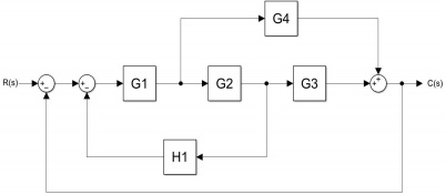
a. Using Mason's Rule method, find the transfer function, C(s)/R(s) for the block diagram shown in Figure 1. The transfer function for the system represented by the block diagram is,
T(s) = C(s)/R(s) = ∑iΡiΔi/Δ
Where,
i = number of forward paths
Pi = the ith forward-path gain
Δ = 1 - ∑ loop gains + ∑ non-touching loop gains taken two at a time
Δi = Δ - ∑ loop gain terms in that touch the ith forward path.
Your answer should be in terms Δ of G1, G2, G3, G4 and H1
b. Write a MATLAB program to compute the transfer function T(s) of the closed-loop system,
T(s) = C(s)/R(s)
Your answer should include a copy of the program listing (*. m file or *.mlx file) and a copy of the step response plot.
Create a Simulink model of the multiple-loop feedback control system shown in Figure 1, using the system parameters given in Table 1. Use a Step Block (Simulink Library Browser/Simulink/Sources) for the input R(s), setting block parameters: Step time: 0, Initial value: 0 and Final Value: 1. Use a Scope Block (Simulink Library Browser/ Simulink/Commonly Used Blocks) to display the output signal C(s) with respect to time. Set the simulation stop time to 30 and run the simulation. Compare the unity step response of the system to the unity step response obtained in Part (b).
Your answer should include a copy of a correctly labelled Simulink model, a copy of the model step response plot showing only the output signal C(s), and a brief comment that compares the two step response plots obtained from Part (b) and Part (c).
QUESTION 2
Consider the following loop transfer function of a system:
D(s) = 1.248 (s+2)/(0.2s + 1)(6s + 3)
Calculate the DC gain of the system and provide your answer in decibels.
Identify the position of the system poles and zeros, using MATLAB instructions to confirm your answer.
Identify the position of each cut-off frequency.
Use the information from Parts (a) to (c) above to sketch the Bode plot of the frequency response (magnitude and phase). Clearly show each cut-off frequency, asymptote plots, and an approximate Bode plot.
Use MATLAB instructions to create a Bode plot of the frequency response of the system and compare the approximate Bode plot derived in Part (d).
QUESTION 3
Consider the feedback control system shown in Figure 2.
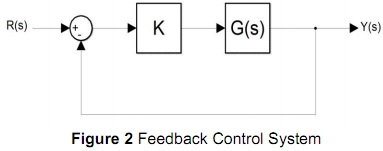
The transfer function G(s) is given,
T(s) = C(s)/R(s) = KG(s)/1+KG(s)
And K is a proportional controller.
To find the value of the controller gain K for which the closed-loop system is marginally stable using the Routh-Hurwitz criterion, you need to:
Clearly identify the system characteristic equation.
Include a completed Routh array.
Provide a statement that clearly identifies the values of the controller gain when the closed-loop system is marginally stable.
Include calculations for each element in the Routh array.
Once you have the characteristic equation and the completed Routh array, you can determine the value of the controller gain K for marginal stability
a. Create a Simulink model of the closed-loop system, using the value of the proportional controller determined in Part (a), and plot the system's step response to demonstrate marginal stability.
QUESTION 4
Consider the loop transfer function of a system as given below:
L(s) = 1/(s+3)(s+9)(s+12)
a. Construct the root-locus plot, illustrating all the steps to determine each part of the root-locus plot.
b. Use MATLAB to plot the root locus and find the maximum proportional gain before the closed-loop system becomes unstable with unity negative feedback.
learning outcomes
C1. Apply knowledge of mathematics, statistics, natural science and engineering principles to the solution of complex problems. Some of the knowledge will be at the forefront of the particular subject of study.
C2. Analyse complex problems to reach substantiated conclusions using first principles of mathematics, statistics, natural science and engineering principles.
C3. Select and apply appropriate computational and analytical techniques to model complex problems, recognising the limitations of the techniques employed.
C5. Design solutions for complex problems that meet a combination of societal, user, business and customer needs as appropriate. This will involve consideration of applicable health and safety, diversity, inclusion, cultural, societal, environmental and commercial matters, codes of practice and industry standards.
C6. Apply an integrated or systems approach to the solution of complex problems. C12. Use practical laboratory and workshop skills to investigate complex problems.