Reference no: EM132395411

Assignment

Answer the questions in both sections below.

Section 1: Election Prediction Based on Betting Markets

In the book, class, and tutorials, we studied the prediction of election outcomes using polls. In this section, we study the prediction of election outcomes based on betting markets. In particular, we analyze data for the 2008 US presidential election from an online betting company, called Intrade. At Intrade, people trade contracts such as ‘Obama to win the electoral votes of Florida.' Each contract's market price fluctuates based on its sales. Why might we expect betting markets like Intrade to accurately predict the outcomes of elections or of other events? Some argue that the market can aggregate available information efficiently. In this exercise, we will test this efficient market hypothesis by analyzing the market prices of contracts for Democratic and Republican nominees' victories in each state. The data file is available in CSV format as intrade08.csv. The variables in these datasets are:

Name             Description
day               Date of the session
statename      Full name of each state (including District of Columbia in 2008)
state             Abbreviation of each state (including District of Columbia in 2008)
PriceD            Closing price (predicted vote share) of Democratic Nominee’s market
PriceR            Closing price (predicted vote share) of Republican Nominee’s market
VolumeD         Total session trades of Democratic Party Nominee’s market
VolumeR         Total session trades of Republican Party Nominee’s market

Each row represents daily trading information about the contracts for either the Democratic or Republican Party nominee's victory in a particularstate. We will also use the election outcome data in the file pres08.csv with variables:

Name             Description
state.name     Full name of state
state             Two letter state abbreviation
Obama           Vote percentage for Obama
McCain           Vote percentage for McCain
EV                 Number of electoral college votes for this state

You may also use poll data from 2008 in the file ‘polls08.csv. The variables in the polling data are:

Name            Description
state            Abbreviated name of state in which poll was conducted
Obama          Predicted support for Obama (percentage)
Romney         Predicted support for Romney (percentage)
Pollster         Name of organization conducting poll
middate        Middle of the period when poll was conducted

Question 1

Use the market prices on the day before the election to predict the 2008 election outcome. To do this, subset the data such that it contains the market information for each state and candidate only on the day before the election. Note that in 2008 the election day was November 4. Compare the closing prices for the two candidates in a given state and classify a candidate whose contract has a higher price as the predicted winner of that state. Which states were misclassified? (It is sufficient to only report the misclassified states.) How does this compare to the classification by polls presented in the chapter?

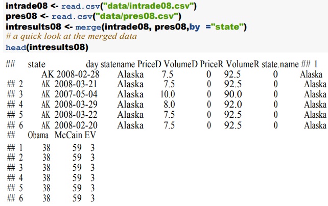
To get you started, here is the code for loading and merging the data:

Question 2

How do the predictions based on the betting markets change over time? Use the classification procedure as above on each of the last 90 days of the 2008 campaign rather than just the day before the election. (Hint: Use a loop.) Plot the predicted number of electoral votes for the Democratic party nominee overthis 90-day period. The resulting plot should also indicate the day of the election and the actual election result. (Hint: Use abline() for these.) Note that in 2008, Obama won 365 electoral votes. Briefly comment on the plot.

Question 3

Repeat the previous exercise but this time use the seven-day moving-average price, instead of the daily price, for each candidate within a state. (Hint: This can be done by recycling code from the previous answer, with some changes inside the loop.) For a given day, we take the average of the Session Close prices within the past seven days (including that day). To answer this question, we must first compute the seven-day average within each state. Next, we sum the electoral votes for the states Obama is predicted to win. Using the tapply() function will allow us to efficiently compute the predicted winner for each state on a given day.

Question 4

Create a similar plot for 2008 state-wide poll predictions using the data file polls08.csv. Notice that polls are not conducted daily within each state. Therefore, within a given state for each of the last 90 days of the campaign, we compute the average margin of victory from the most recent poll(s) conducted. If multiple polls occurred on the same day, average these polls. Based on the most recent predictions in each state, sum Obama's total number of predicted electoral votes. One strategy to answer this question is to program two loops - an inner loop with 51 iterations for each state and an outer loop with 90 iterations for each day. (Hint: You can use a counter in the inner loop to collect electoral votes per state, and in the outer loop save/assign the result and reset the counter.)

Question 5

What is the relationship between the price margins of the Intrade market and the actual margin of victory? Using only the market data from the day before the election in 2008, regress Obama's actual margin of victory in each state on Obama's price margin from the Intrade markets. Considering only the trading one day from the election, predict the actual electoral margins from the trading margins using a linear model. Does it predict well? How would you visualize the predictions and the outcomes together? (Hint: Because we only have one predictor you can use abline().) Similarly, in a separate analysis, regress Obama's actual margin of victory on the Obama's predicted margin from the latest polls within each state. Interpret the results of these regressions.

Question 6

Even efficient markets are not omniscient. Information comes in about the election every day and the market prices should reflect any change in information that seem to matter to the outcome. We can examine how and about what the markets change their minds by looking at which states they are confident about, and which they update their ‘opinions' (i.e. their prices) about. Over the period before the election, let'ssee how prices for each state are evolving. We can get a compact summary of price movement by fitting a linear model to Obama's margin for each state over the 20 days before the election. We will summarise price movement by the direction (up or down) and rate of change (large or small) of price over time. (This is basically also what people in finance do.) Start by plotting Obama's margin in West Virginia against the number of days until the election and modeling the relationship with a linear model. (Hint: West Virginia is 50th on the alphabetical list of state names.) Use the last 20 days. Show the model's predictions on each day and the data. What does this model's slope coefficient tells us about which direction the margin is changing and also how fast it is changing? Then do it for all states and collect the slope coefficients to see how volatile the state estimates are. Show the distribution of these slopes with a histogram.

Question 7

Now predict the winner of the election one week before the election using the Intrade data. To do so, first use the two weeks before that moment to fit state level linear models, then use those models to predict what will happen in each state. How well does the model do predicting the election outcome?

Section 2: Immigration Attitudes

Why do the majority of voters in the U.S. and other developed countries oppose increased immigration? According to the conventional wisdom and many economic theories, people simply do not want to face additional competition on the labor market (economic threat hypothesis). Nonetheless, most comprehensive empirical tests have failed to confirm this hypothesis and it appears that people often support policies that are against their personal economic interest. At the same time, there has been growing evidence that immigration attitudes are rather influenced by various deep-rooted ethnic and cultural stereotypes (cultural threat hypothesis). Given the prominence of workers' economic concerns in the political discourse, how can these findings be reconciled?

This exercise is based in part on Malhotra, N., Margalit, Y. and Mo, C.H., 2013. "Economic Explanations for Opposition to Immigration: Distinguishing between Prevalence and Conditional Impact." American Journal of Political Science, Vol. 38, No. 3, pp. 393-433.

The authors argue that, while job competition is not a prevalent threat and therefore may not be detected by aggregating survey responses, its conditional impact in selected industries may be quite sizable. To test their hypothesis, they conduct a unique survey of Americans' attitudes toward H1B visas. The plurality of H-1B visas are occupied by Indian immigrants, who are skilled but ethnically distinct, which enables the authors to measure a specific skill set (high technology) that isthreatened by a particular type of immigrant (H-1B visa holders). The data set immig.csv has the following variables:

Name                     Description
age                       Age (in years)
female                   1 indicates female; 0 indicates male
employed               1 indicates employed; 0 indicates unemployed
nontech.whitcol      1 indicates non-tech white-collar work (e.g., law)
tech.whitcol           1 indicates high-technology work
expl.prejud             Explicit negative stereotypes about Indians (continuous scale, 0-1)
impl.prejud             Implicit bias against Indian Americans (continuous scale, 0-1)
h1bvis.supp            Support for increasing H-1B visas (5-point scale, 0-1)
indimm.supp            Support for increasing Indian immigration (5-point scale, 0-1)

The main outcome ofinterest (h1bvis.supp) was measured as a following survey item: "Some people have proposed that the U.S. government should increase the number of H-1B visas, which are allowances for U.S. companies to hire workers from foreign countries to work in highly skilled occupations(such as engineering, computer programming, and high-technology). Do you think the U.S. should increase, decrease, or keep about the same number of H-1B visas?" Another outcome (indimm.supp) similarly asked about the "the number of immigrants from India." Both variables have the following response options: 0 = "decrease a great deal", 0.25 = "decrease a little", 0.5 =
"keep about the same", 0.75 = "increase a little", 1 = "increase a great deal".

To measure explicit stereotypes (expl.prejud), respondents were asked to evaluate Indians on a series of traits: capable, polite, hardworking, hygienic, and trustworthy. All responses were then used to create a scale lying between 0 (only positive traits of Indians) to 1 (no positive traits of Indians). Implicit bias (impl.prejud) is measured via the Implicit Association Test (IAT) which is an experimental method designed to gauge the strength of associations linking social categories (e.g., European vs Indian American) to evaluative anchors (e.g., good vs bad). Individual who are prejudiced against Indians should be quicker at making classifications of faces and words when European American (Indian American) is paired with good (bad) than when European American (Indian American) is paired with bad (good).

Question 1

Start by examining the distribution of immigration attitudes (as factor variables). What is the proportion of people who are willing to increase the quota for high-skilled foreign professionals (h1bvis.supp) orsupport immigration from India (indimm.supp)? Now compare the distribution oftwo distinct measures of cultural threat: explicitstereotyping about Indians (expl.prejud) and implicit bias againstIndian Americans(impl.prejud). In particular, create a scatterplot, add a linear regression line to it, and calculate the correlation coefficient. Based on these results, what can you say about their relationship?

Question 2

Compute the correlations between all four-policy attitude and cultural threat measures. Do you agree that cultural threat is an important predictor of immigration attitudes as claimed in the literature?

If the labor market hypothesis is correct, opposition to H-1B visas should also be more pronounced among those who are economically threatened by this policy such as individuals in the hightechnology sector. At the same time, tech workers should not be more or less opposed to general Indian immigration because of any economic considerations. First, regress H-1B and Indian immigration attitudes separately on the indicator variable for tech workers(tech.whitcol). Do the resultssupport the hypothesis? Isthe relationship different from the one involving cultural threat and, if so, how?

Question 3

When examining hypotheses, it is always important to have an appropriate comparison group. One may argue that comparing tech workers to everybody else as we did in Question 2 may be problematic due to a variety of confounding variables (such as skill level and employment status).

First, create a single factor variable group which takes a value of tech if someone is employed in tech, whitecollarifsomeone is employed in other "white-collar" jobs (such as law or finance), other if someone is employed in any other sector, and unemployed if someone is unemployed. Then, compare the support for H-1B across these conditions by using linear regression. Interpret the results: is this comparison more or less supportive of the labor market hypothesis than the one in Question 2?

Now, one may also argue that those who work in the tech sector are disproportionately young and male which may confound our results. To account for this possibility, fit another linear regression but also include age and female as pre-treatment covariates (in addition to group). Does it change the results and, if so, how?

Finally, fit a linear regression model with all threat indicators (group, expl.prejud, impl.prejud) and calculate its R2. How much of the variation is explained? Based on the model fit, what can you conclude about the role of threat factors?

Question 4

Besides economic and cultural threat, many scholars also argue that gender is an important predictor of immigration attitudes. While there is some evidence that women are slightly less opposed to immigration than men, it may also be true that gender conditions the very effect of other factors such as cultural threat. To see if it is indeed the case, fit a linear regression of H-1B support on the interaction between gender and implicit prejudice. Then, create a plot with the predicted level of H-1B support (y-axis) across the range of implicit bias (x-axis) by gender. Considering the results, would you agree that gender altersthe relationship between cultural threat and immigration attitudes?

Age is another important covariate. Fit two regression models in which H-1B support is either a linear or quadratic function of age. Compare the results of both models by plotting the predicted levels of support (y-axis) across the whole age range (x-axis). Would you say that people become more opposed to immigration with age?

Question 5

To corroborate your conclusions with regard to cultural threat, create separate binary variables for both prejudice indicators based on their median value (1 if >than the median) and then compare average H-1B and Indian immigration attitudes (as numeric variables) depending on whether someone is implicitly or explicitly prejudiced (or both). What do these comparisons say about the role of cultural threat?

What about the role of economic threat? One may argue that tech workers are simply more or less prejudiced against Indians than others. To account for this possibility, investigate whether economic threat is in fact distinguishable from cultural threat as defined in the study. In particular, compare the distribution of cultural threat indicator variable using the Q-Q plot depending on whethersomeone isin the high-technology sector. Would you conclude that cultural and economic threat are really distinct?