Reference no: EM132371788

Q1) Potential outcomes, DAGs, and sub-classification

• Consider the simple hypothetical example in Table 1.  This example involves four units (patients) and two possible medical procedures labeled 0 (Drug) and 1 (Surgery).  Assuming SUTVA, Table 1 displays each patient’s potential outcomes in terms of years of post-treatment survival under each treatment.

Table 1: Perfect doctor example

a. Calculate the average treatment effect for surgery compared to drug? Which type of intervention is more effective on average?

b. Suppose that there is some “perfect doctor” who through expertise or magic knows each patient’s potential outcomes and then chooses the optimal treatment for each patient. If she assigns each patient to the treatment more beneficial for that patient, which patients will receive surgery, and which will receive the drug treatment? Calculate the average treatment effect for the group who received surgery. Calculate the average treatment effect for the group who received drug treatment.

c. Assume that the “perfect doctor” has assigned each patient to his or her own optimal treatment. Calculate the simple difference in means for surgery using that observable information. How does this differ from the average treatment effect?

d. Decompose the simple difference in means into the two biases discussed in class (selection bias and heterogeneous treatment effect bias) plus the average treatment effect. In your own words, what is the cause of the difference between the “real” average treatment effect of surgery and the difference in means?

e. What is the “fundamental problem of causal inference” in this context?

f. Take a coin and flip it ten times. If heads on the first flip, unit 1 is assigned to drug and if tails is assigned to surgery. If heads on the second flip, unit 2 is assigned to drug and if tails is assigned to surgery. And so on. Calculate the estimated average treatment effect and compare it with your answers.

Q2)  Use Figure 2 for the following questions.  In all four DAGs (a-d), X is a binary treatment variable and Y is the outcome variable, U and V are unobservable. S, Z, X and Y are all observable (in your data).

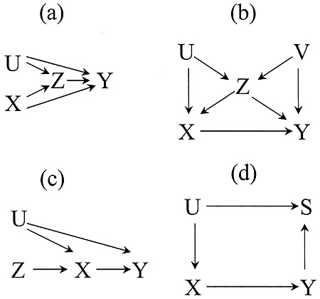
Figure 2: Four DAG examples

a. For each DAG, write down all backdoor paths from X to Y and indicate whether they are open or closed.  Write down a conditioning strategy that satisfies the backdoor criterion.  If one does not exist, why does it not exist? 

Q3  Titanic dataset

Use “titanic3.csv” for the following questions. Read “titanic3_readme.pdf” for information about each variable in the dataset. The SS Titanic is a tragic sinking in maritime history, and as the story is well known, I won’t repeat it here.  For our purposes, we will focus on efforts to estimate the average causal effects of individual attributes on access to lifeboats, and therefore survival.

Individuals who did not enter a lifeboat during the ship’s sinking were almost certainly doomed due to the frigid temperature of the Atlantic Ocean that morning. Given the scarcity of lifeboats, the Crew and Passengers used the maritime social norm, “Women and Children First”, to allocate lifeboats to passengers and crew.  But it is plausible that other individual attributes, such as first class status, had a causal effect on survival given the proximity of first class passengers to the lifeboats themselves, as well as other possible mechanisms (e.g., bribes).

A) Assume that gender and age perfectly block all backdoors connecting “first class” and “survival”. What are the identifying assumptions that must be made for us to use subclassification/stratification to estimate the causal effect of first class on survival? Explain each in plain English, as well as using the notation from class.

B) Calculate the effect of first class on survival using naïve average treatment effect. Explain why you think this is biased. Would such an analysis suffer from selection bias or reverse causality? If so, why?

C) Suppose that the data set did not contain the `boat’ variable, but still estimated the effect of passenger class on survival without the knowledge of whether a passenger was placed into a lifeboat. What direction would you expect the omitted variable to bias the estimate of first class on survival?

D) Calculate the effect of first class on survival using a stratification variable, S, that takes on four values: 1 for male child, 2 for male adult, 3 for female child, 4 for female adult. Define a child any individual younger than 15. All adults, therefore, are 15 or older. Compare the naïve ATE with the weighted ATE and weighted average treatment effect on the treatment group.

E) Say that instead of using only two values for age (e.g., child and adult), you used all values of age. Can you use subclassification to estimate the average causal effects? Why/why not?

F) What if individuals had actually lied about their age during the sinking of the ship? Although records contain the actual age of individuals on the vessel, their reported age during the sinking might have differed. How would this impact the analyses in (D) and (E)?

Build a dataset.

Go to ICPSR (create an account if you don’t already have one) and download “Uniform Crime Reporting (UCR) Program Data: Raw Data” uploaded by Jacob Kaplan. This should be a zipfile of monthly data from 1974-2016. You must download monthly data!

Cleaning the UCR data

You can choose the order in which you to the following steps. I recommend writing a loop function to do this.

• Select out the following variables:

state year fips_state_county_code actual_index_property actual_index_violent ori population

Only keep data from California (fips code = 06)

• Rename actual_index_property to property_crime and actual_index_violent to violent_crime

• Convert the data from monthly to annual (sum property_crime and violent_crime)

• Drop all agencies that do not report their population (or report a population of 0)

• Convert data from agency (ori) to county level (sum property_crime and violent_crime population)

• Paste together the data from 2010 – 2014

• Create variables for property_crime_rate per 10,000 in the papulation property_crime_rate and violent_crime_rate per 10,000 in the papulation

If you are using Stata, save the clean data to a data file called UCR.dta, (use the replace command)

Q4 )

Download American Community Survey (ACS) data at the county level for 2010-2014. You only need data from California (fips code = 06), you can download only data from CA or download for all states and only keep data from CA.

• You can use the census website or IPUMS (I think IPUMS is easier, but you have to create an account)

• Download the following variables: STATEFIP COUNTYFIP SEX POVERTY SCHOOL RACWHT RACBLK

• Convert data to the county-year level and create variables for the following:

Proportion of the population that is white, proportion of the population that is black, proportion of the population that is in poverty and proportion of the population that has a bachelor’s degree.

• Merge together the ACS data and the UCR data

• Only keep counties that are in both data sets

11. Create a summary statistics table

• Include: property_crime_rate, violent_crime_rate, portion of the population that is white, black, in poverty and that have a bachelor’s degree.

Reading - CAUSAL INFERENCE: THE MIXTAPE (V. 1. 7 ) By 8 Scott Cunningham

Attachment:- Assignment-medical procedures.rar