Graphical representation of various returns, Microeconomics

Assignment Help:

Graphical Representation of Various Returns:

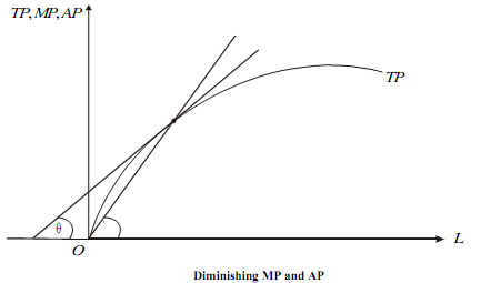
Diminishing Returns: If the TP curve is as shown in the adjacent Figure, then the MPL given by tanθ  is throughout less than the APL given by tanθ.  


1133_Graphical Representation of Various Returns.png

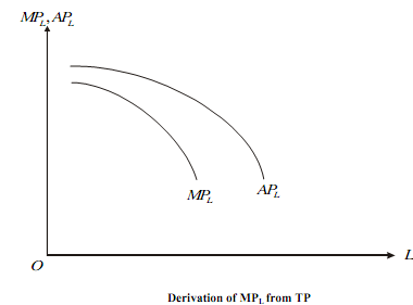
As APL is falling from the relation between MP and AP, MP < AP we have the adjoining Figure.   

195_Graphical Representation of Various Returns1.png

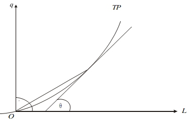
Increasing Returns Here APL rises and tan  < tanθ , for all L. Therefore, MP > AP. This is shown in the adjacent Figure.  


677_Graphical Representation of Various Returns2.png


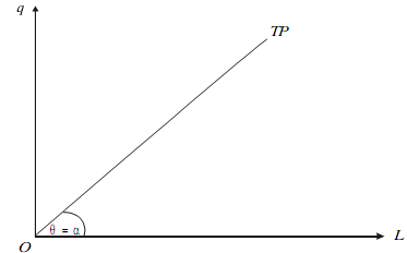
Constant Returns Here, APL is constant and tanθ  = tan , therefore, MPL = APL as is shown by a horizontal straight line in the next Figure(a,b)   

2493_Graphical Representation of Various Returns3.png

The TP curve is such that upto point A, MP is rising and so is AP and MP > AP, as shown in the diagram below. Beyond point A, MP falls but AP rises, till the two are equated at point B. At B, AP is maximised. AP falls beyond the point B. At point C, the TP curve flattens out and therefore, MP = 0. Beyond C, MP is negative and AP is falling. Therefore, in the case of non-proportional return, both MP and AP rise, initially. MP reaches a maximum earlier than AP. When they both are equated, AP is maximised. Finally, there is a situation where both are falling. Depending on the nature of MP and AP, the production process can be divided into three stages - I, II, and III, as shown in Figure. 

Characteristics of the three stages are : 

Stage I: MP > 0, AP rising, thus MP > AP 

Stage II: MP > 0, AP falling, thus MP < AP 

Stage III: MP < 0, AP falling  

In stage I, by adding one more unit of L, the producer can increase the average productivity of all the units. Thus, it would be unwise for the producer to stop production in this stage. 

In stage III, MP < 0, so that by reducing the L input, the producer can increase the total output and save the cost of a unit of L. Therefore, it is impractical for a producer to produce in this stage. 

Hence, stage II represents the economically meaningful range. This is so because here MP > 0 and AP > MP. So that an additional L input would raise the total production. Besides, it is in this stage that the TP reaches a maximum.  


Related Discussions:- Graphical representation of various returns

Exchange rate policy, Exchange Rate Policy: LERMS, a dual exchange ra...

Exchange Rate Policy: LERMS, a dual exchange rate system, was introduced in the Budget for 1992-93. Under this system, 40 per cent of foreign exchange earnings were to be sur

Market failure, Ask question using health care as an example explain how ma...

Ask question using health care as an example explain how markets fail due to different types of externalities arising from jointness in production and consumption

Determine the price charged by the profit maximizing cartel, In an industry...

In an industry with two firms, represent the outputs for these single product firms as q 1 and q 2 . The two firms decide to form a cartel and set their levels of output to maxim

Consumer choice involving risk.., why risk averse consumers pay premium for...

why risk averse consumers pay premium for insurance to convert an uncertain outcome to a certain one?

#t, what are the relevance of economics to most business today??

what are the relevance of economics to most business today??

Illustrate about the elasticity of substitution, Illustrate about the elast...

Illustrate about the elasticity of substitution. The Elasticity of Substitution: The technical substitution’s marginal rate measures the slope of an isoquant. As well the el

Lending capacity of cash, Assume the banking system contains: Total Rese...

Assume the banking system contains: Total Reserves                         $ 80 billion Transactions Deposited          $800 billion Cash held by public                 $1

Production possibility curve, draw a production possibility frontier task u...

draw a production possibility frontier task using the graph and value and identity the pareto efficent and inefficient point and the marginal oppotunity cost of x for each point of

Opertunity cost, how do you calculate opportunity cost

how do you calculate opportunity cost

Write Your Message!

Captcha
Free Assignment Quote

Assured A++ Grade

Get guaranteed satisfaction & time on delivery in every assignment order you paid with us! We ensure premium quality solution document along with free turntin report!

All rights reserved! Copyrights ©2019-2020 ExpertsMind IT Educational Pvt Ltd