Macroeconomics Assignment Help >> The Neo-Classical Synthesis Assignment Help

The neo-classical synthesis

Introduction

The neo-classical synthesis is a synthesis of the classical model and the Keynesian model. In short, it states that the Keynesian model is correct in the short run while the classical analysis is correct in the long run.

Let us consider a concrete example. According to the Keynesian model, an increase in G will increase Y and reduce unemployment. In the classical model, an increase in G will have no effect at all on Y and unemployment. In the neo-classical synthesis, an increase in G will create a temporary increase in Y but Y will return to its original value after some time.

To justify the neo-classical synthesis, it is helpful to identify the problem with the classical model in the short run and the problem with the Keynesian model in the long run. As for the classical model in the short run, we concluded that within this model, it is difficult to explain deep recessions with high involuntary unemployment. In the long run, it is more reasonable to believe that that the economy can get out of the recession by itself. The problem with the Keynesian model in the long run, as we will see, is the assumption of a stable Phillips curve.

The various Phillips curves


The augmented Phillips curve

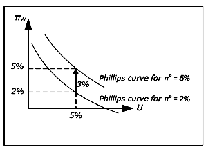
Remember that the Phillips curve, as it was incorporated into the Keynesian model, assumed a stable relationship between unemployment and wage inflation: for a given level of unemployment (say U = 5%), a given level of wage inflation would apply (say π_w = 4%). As U increased, π_w would fall and Vice versa.

Mathematically, the Phillips curve may be described by a decreasing function f as π_w = f(U). In the neo-classical synthesis, expected inflation is added and π_w = f(U) + π^e. To justify this amendment, imagine U = 5% and π_w = 4% (so that we are on the Phillips curve) and the expected inflation rises from 4% to 6%. Since employees care about real wages, it is reasonable to assume that πW will increases as well (for a given U) and the Phillips curve will shift upwards.

The augmented Phillips curve



According to the synthesis, the Phillips curve must be drawn for a given value of π_e and it must be shifted upwards (downwards) as If increases (decreases). When the position of the Phillips curve is allowed to depend on If, is called the augmented Phillips curve (or the expectations-augmented Phillips curve). This amendment to the Phillips curve is actually a consequence of a criticism of the traditional Phillips curve and the Keynesian model from the late 1960's (the Keynesian - Monetarism debate).

Money illusion

An important argument for the augmentation has to do with the concept of money illusion. Money illusion means that you care about nominal rather than real amounts. Imagine that your salary increases by 20% over one year. Does this mean that you can increase your consumption? The answer is that it depends on the inflation. If inflation is 20%, you can consume as much as you did before. You must actually decrease you consumption if inflation exceeds 20%. We say that you have suffer from money illusion if you believe that you are better off if your salary increases by 20% while prices also increase by 20%. A higher nominal salary may create the "illusion" that you are richer.

If employees suffer from money illusion they will only care about nominal wage increases, expected inflation will not matter and there is no reason for the traditional Phillips curve not to hold. If, however, they do not suffer from money illusion, π_w must depend on both U and π_e and the augmented Phillips curve is more realistic.

The long-run Phillips curve

The augmented Phillips curve has an important consequence: the long-run Phillips curve must be vertical.

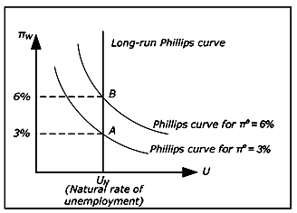
To realize this, start by drawing a Phillips curve for e = 3%. The only point on this curve that may apply in the long run is π_w= 3% (point A). For example, π_w= 2% and π_e = 3% is not consistent with equilibrium in the long run as there is no level of inflation which is consistent with these values. π = 3% is not possible as real wages would go to zero. π= 2% is not possible since it would be unreasonable to continue to expect 3% inflation if inflation each year was 2%.

According to the neo-classical synthesis, we may temporarily be anywhere on the lower Phillips curve when π_e = 3 %, but the economy must eventually return to point A (as long π_e = 3 %)

Now draw a Phillips curve for π_e = 6%. Again, on this curve there is only one point is consistent with equilibrium in the long run and that is the point where π_w = 6% (point B). This point must be exactly above A as the new curve must be exactly three units above the first curve.

If we draw all possible Phillips curves, we see that all points consistent with long run equilibrium must lie on a vertical curve and this curve is called the long-run Phillips curve. In the long run, the economy must return to this curve. This means that in the long run, there is no relation between inflation and unemployment. In the long term, the economy returns to the natural unemployment rate as in the classical model.

Summary of the Phillips curves


In the neo-classical synthesis, the augmented Phillips curve is called the short-run Phillips curve. It is assumed to be stable as long as expectations of future inflation do not change. To summarize, we have three Phillips curves:

• The traditional Phillips curve. π_w = f(U) and the same downward sloping relationship applies to both the short and the long run.

• The short-run Phillips curve (SPC). π_w = f(U) + π_e and the curve is valid only in the short run (SPC = Short-run Phillips Curve).

• The long-run Phillips curve (LPC). π_w = π_M, U = U_N and there is no relationship between w and U (UN is the natural rate of unemployment).

The classical model and the long-term Phillips curve

In the classical model, L and the real wage are determined from equilibrium conditions in the labor market. Land W / P, therefore, are only affected by the marginal product of labor (which determines the demand for labor) and by the utility function of the employees (which determines the supply of labor). All unemployment is voluntary and L, U or W/P are all affected by exogenous variables only.

In the classical model, inflation is determined solely by the growth in the money supply M. From the quantity theory of money, M• V = P: Y and if the growth rate of M is π_M, then P must increase by the same rate as V and Yare constant. From the quantity theory we can conclude that π= π_M must hold. The relationship M•V = P•Y is therefore sometimes called the quantity theory in levels while π = π_Mis called the quantity theory in rates.

In the classical model, inflation is balanced and w= (real wage is constant). Since π= π_M, we have π= π_M =π_w. As U is not affected by any endogenous variables, there is no relationship between π_w och U in the classical model and the vertical LPC applies even in the short run. The position on the LPC determined by π_M.

Unlike the neo-classical synthesis, where the economy temporarily may depart from LPC, the economy must always be on the LPC in the classical model.

Email based Macroeconomics Homework Help & Assignment Help

We offer online solutions for macroeconomics subject’s topics neo-classical synthesis , Phillips curve theory and concepts. We offer email based assignment help, homework help and project help in macroeconomics subject. Send your assignment’s problems at [email protected] and get quote for a solution which is economical in student’s point of view. You can post your assignment work in the form given below.