Reference no: EM13869916
1. Which value of r indicates a stronger correlation: r = 0.755 or r = -0.867? Explain your reasoning.=
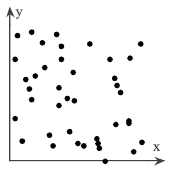
2. The scatter plot of a paired data set is shown. Determine whether there is a perfect positive linear correlation, a strong positive linear correlation, a perfect negative linear correlation, a strong positive linear correlation, a perfect negative linear correlation, a strong negative linear correlation, or no linear correlation between the variables.
3. Identify the explanatory variable and the response variable.
A teacher wants to determine if the type of textbook used by her students can be used to predict the students' test scores.
4. For the following data
a. Display the data in a scatter plot.
b. Calculate the correlation coefficient r.
c. Make a conclusion about the type of correlation.
The ages (in years) of 6 children and the number of words in their vocabulary
|
Age, x
|
1
|
2
|
3
|
4
|
5
|
6
|
|
Vocabulary size, y
|
300
|
750
|
1450
|
1450
|
1700
|
2700
|
5. The budget (in millions of dollars) and worldwide gross (in millions of dollars) for eight movies are shown below. Complete parts (a) through (c).
|
Budget, x
|
206
|
202
|
198
|
198
|
180
|
176
|
174
|
168
|
|
Gross, y
|
1218
|
1807
|
1016
|
661
|
661
|
426
|
344
|
269
|
a. Display the data in a scatter plot.
b. Calculate the correlation coefficient r.
c. Make a conclusion about the type of correlation.
6. The weights (in pounds) of 6 vehicles and the variability of their braking distances (in feet) when stopping on a dry surface are shown in the table. Can you conclude that there is a significant linear correlation between vehicle weight and variability in braking distance on a dry surface? Use α = 0.01.
|
Weight, x
|
5910
|
5380
|
6500
|
5100
|
5840
|
4800
|
|
Variability in braking distance, y
|
1.75
|
1.93
|
1.89
|
1.64
|
1.63
|
1.50
|
Data Table
|
|
Level of
confidence, c
|
0.50
|
0.80
|
0.90
|
0.95
|
0.98
|
0.99
|
|
|
One tail, a
|
0.25
|
0.10
|
0.05
|
0.025
|
0.01
|
0.005
|
|
d.f.
|
Two tails, a
|
0.50
|
0.20
|
0.10
|
0.05
|
0.02
|
0.01
|
|
1
|
|
1.000
|
3.078
|
6.314
|
12.706
|
31.821
|
63.657
|
|
2
|
|
0.816
|
1.886
|
2.920
|
4.303
|
6.965
|
9.925
|
|
3
|
|
0.765
|
1.638
|
2.353
|
3.182
|
4.541
|
5.841
|
|
4
|
|
0.741
|
1.533
|
2.132
|
2.776
|
3.747
|
4.604
|
|
5
|
|
0.727
|
1.476
|
2.015
|
2.571
|
3.365
|
4.032
|
|
6
|
|
0.718
|
1.440
|
1.943
|
2.447
|
3.143
|
3.707
|
|
7
|
|
0.711
|
1.415
|
1.895
|
2.365
|
2.998
|
3.499
|
|
8
|
|
0.706
|
1.397
|
1.860
|
2.306
|
2.896
|
3.355
|
|
9
|
|
0.703
|
1.383
|
1.833
|
2.262
|
2.821
|
3.250
|
|
10
|
|
0.700
|
1.372
|
1.812
|
2.228
|
2.764
|
3.169
|
|
11
|
|
0.697
|
1.363
|
1.796
|
2.201
|
2.718
|
3.106
|
|
12
|
|
0.695
|
1.356
|
1.782
|
2.179
|
2.681
|
3.055
|
|
13
|
|
0.694
|
1.350
|
1.771
|
2.160
|
2.650
|
3.012
|
|
14
|
|
0.692
|
1.345
|
1.761
|
2.145
|
2.624
|
2.977
|
|
15
|
|
0.691
|
1.341
|
1.753
|
2.131
|
2.602
|
2.947
|
|
16
|
|
0.690
|
1.337
|
1.746
|
2.120
|
2.583
|
2.921
|
|
17
|
|
0.689
|
1.333
|
1.740
|
2.110
|
2.567
|
2.898
|
|
18
|
|
0.688
|
1.330
|
1.734
|
2.101
|
2.552
|
2.878
|
|
19
|
|
0.688
|
1.328
|
1.729
|
2.093
|
2.539
|
2.861
|
|
20
|
|
0.687
|
1.325
|
1.725
|
2.086
|
2.528
|
2.845
|
|
21
|
|
0.686
|
1.323
|
1.721
|
2.080
|
2.518
|
2.831
|
|
22
|
|
0.686
|
1.321
|
1.717
|
2.074
|
2.508
|
2.819
|
|
23
|
|
0.685
|
1.319
|
1.714
|
2.069
|
2.500
|
2.807
|
|
24
|
|
0.685
|
1.318
|
1.711
|
2.064
|
2.492
|
2.797
|
|
25
|
|
0.684
|
1.316
|
1.708
|
2.060
|
2.485
|
2.787
|
|
26
|
|
0.684
|
1.315
|
1.706
|
2.056
|
2.479
|
2.779
|
|
27
|
|
0.684
|
1.314
|
1.703
|
2.052
|
2.473
|
2.771
|
|
28
|
|
0.683
|
1.313
|
1.701
|
2.048
|
2.467
|
2.763
|
|
29
|
|
0.683
|
1.311
|
1.699
|
2.045
|
2.462
|
2.756
|
|
∞
|
|
0.674
|
1.282
|
1.645
|
1.960
|
2.326
|
2.576
|
7. The following table shows the earnings per share and dividends per share for 10 electric utility companies in a recent year. The linear correlation coefficient is r = 0.336661. At α = 0.05, can you conclude that there is a significant linear correlation between earnings per share and dividends per share?
Data Table
|
|
Level of
confidence, c
|
0.50
|
0.80
|
0.90
|
0.95
|
0.98
|
0.99
|
|
|
One tail, a
|
0.25
|
0.10
|
0.05
|
0.025
|
0.01
|
0.005
|
|
d.f.
|
Two tails, a
|
0.50
|
0.20
|
0.10
|
0.05
|
0.02
|
0.01
|
|
1
|
|
1.000
|
3.078
|
6.314
|
12.706
|
31.821
|
63.657
|
|
2
|
|
0.816
|
1.886
|
2.920
|
4.303
|
6.965
|
9.925
|
|
3
|
|
0.765
|
1.638
|
2.353
|
3.182
|
4.541
|
5.841
|
|
4
|
|
0.741
|
1.533
|
2.132
|
2.776
|
3.747
|
4.604
|
|
5
|
|
0.727
|
1.476
|
2.015
|
2.571
|
3.365
|
4.032
|
|
6
|
|
0.718
|
1.440
|
1.943
|
2.447
|
3.143
|
3.707
|
|
7
|
|
0.711
|
1.415
|
1.895
|
2.365
|
2.998
|
3.499
|
|
8
|
|
0.706
|
1.397
|
1.860
|
2.306
|
2.896
|
3.355
|
|
9
|
|
0.703
|
1.383
|
1.833
|
2.262
|
2.821
|
3.250
|
|
10
|
|
0.700
|
1.372
|
1.812
|
2.228
|
2.764
|
3.169
|
|
II
|
|
0.697
|
1.363
|
1.796
|
2.201
|
2.718
|
3.106
|
|
12
|
|
0.695
|
1.356
|
1.782
|
2.179
|
2.681
|
3.055
|
|
I3
|
|
0.694
|
1.350
|
1.771
|
2.160
|
2.650
|
3.012
|
|
14
|
|
0.692
|
1.345
|
1.761
|
2.145
|
2.624
|
2.977
|
|
15
|
|
0.691
|
1.341
|
1.753
|
2.131
|
2.602
|
2.947
|
|
16
|
|
0.690
|
1.337
|
1.746
|
2.120
|
2.583
|
2.921
|
|
17
|
|
0.689
|
1.333
|
1.740
|
2.110
|
2.567
|
2.898
|
|
18
|
|
0.688
|
1.330
|
1.734
|
2.101
|
2.552
|
2.878
|
|
19
|
|
0.688
|
1.328
|
1.729
|
2.093
|
2.539
|
2.861
|
|
20
|
|
0.687
|
1.325
|
1.725
|
2.086
|
2.528
|
2.845
|
|
21
|
|
0.686
|
1.323
|
1.721
|
2.080
|
2.518
|
2.831
|
|
22
|
|
0.686
|
1.321
|
1.717
|
2.074
|
2.508
|
2.819
|
|
23
|
|
0.685
|
1.319
|
1.714
|
2.069
|
2.500
|
2.807
|
|
24
|
|
0.685
|
1.318
|
1.711
|
2.064
|
2.492
|
2.797
|
|
25
|
|
0.684
|
1.316
|
1.708
|
2.060
|
2.485
|
2.787
|
|
26
|
|
0.684
|
1.315
|
1.706
|
2.056
|
2.479
|
2.779
|
|
27
|
|
0.684
|
1.314
|
1.703
|
2.052
|
2.473
|
2.771
|
|
28
|
|
0.683
|
1.313
|
1.701
|
2.048
|
2.467
|
2.763
|
|
29
|
|
0.683
|
1.311
|
1.699
|
2.045
|
2.462
|
2.756
|
|
co
|
|
0.674
|
1.282
|
1.645
|
1.960
|
2.326
|
2.576
|
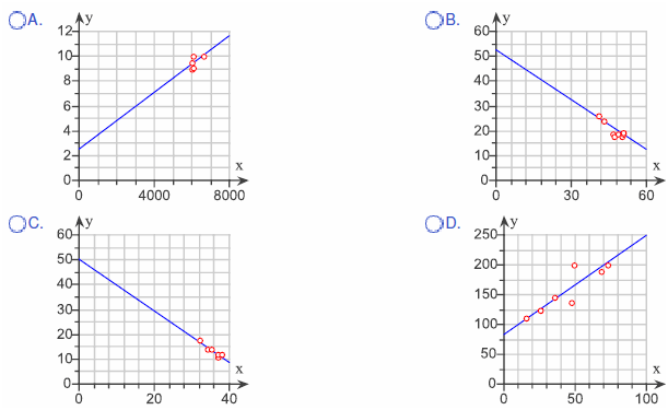
8. Match the regression equation y^ = -0.667x + 52.6 with the approximate graph.
Choose the correct answer below.
9. Find the equation of the regression line for the given data. Then construct a scatter plot of the data and draw the regression line. (Each pair of variables has a significant correlation.) Then use the regression equation to predict the value of y for each of the given x-values, if meaningful. The caloric content and the sodium content (in milligrams) for 6 beef hot dogs are shown in the table below.
|
Calories, x
|
160
|
180
|
130
|
130
|
70
|
190
|
|
Sodium, y
|
420
|
470
|
320
|
360
|
290
|
510
|
a. x = 150 calories
b. x = 100 calories
c. x = 140 calories
d. x = 50 calories
10. Complete parts (a) through (c) using the following data.
|
Row 1
|
1
|
1
|
2
|
3
|
5
|
5
|
5
|
5
|
7
|
7
|
|
Row 2
|
91
|
82
|
81
|
77
|
98
|
71
|
75
|
84
|
57
|
65
|
a. Find the equation of regression line for the given data, letting Row 1 represent the x-values and Row 2 the y-values. Sketch a scatter plot of the data and draw the regression line.
Input the values of the slope and intercept for the regression line when Row 1 represent the x-values.
b. Find the equation of the regression line for the given data, letting Row 2 represent the x-values and Row 1 the y-values. Sketch a scatter plot of the data and draw the regression line.
Input the values of the slope and intercept for the regression line when Row 2 represent the x-values.
c. What effect does the switching the explanatory and response variables have on the regression line?
11. Use the data shown in the table. Replace each x-value and y-value in the table with its logarithm. Find the equation of the regression line for the transformed data. Then construct a scatter plot of (logx, log y) and sketch the regression line with it. What do you notice?
|
x
|
1
|
2
|
3
|
4
|
5
|
6
|
7
|
8
|
|
y
|
466
|
182
|
102
|
36
|
16
|
47
|
36
|
43
|
Find the equation of the regression line of the transformed data.
12. Use the value of the linear correlation coefficient to calculate the coefficient of determination. What does this tell you about the explained variation of the data about the regression line? About the unexplained variation?
r = 0.173
13. The money raised and spent (both in millions of dollars) by all congressional campaigns for 8 recent 2-year periods are shown in the table. The equation of the regression line is y^ = 0.925x + 44.506. Complete parts a and b.
|
Money raised, x
|
452.9
|
665.9
|
731.4
|
779.9
|
775.3
|
1037.7
|
953.8
|
1208.5
|
|
Money spent, y
|
449.1
|
682.1
|
741.2
|
766.7
|
734.2
|
1000.7
|
933.9
|
1158.6
|
a. Find the coefficient of determination and interpret the result.
b. Find the standard error of estimate se and interpret the result.
14. The number of initial public offerings of stocks issued in a 10-year period and the total proceeds of these offerings (in millions) are shown in the table. Construct and interpret a 95% prediction interval for the proceeds when the number of issues is 573. The equation of the regression line is.
y^= 30.936x + 18,283.456.
|
Issues, x
|
404
|
457
|
696
|
489
|
480
|
398
|
63
|
63
|
182
|
154
|
|
Proceeds, y
|
17,929
|
29,081
|
43,458
|
31,582
|
35,269
|
35,857
|
20,789
|
12,354
|
31,678
|
29,588
|
Construct and interpret a 95% prediction interval for the proceeds when the number of issues is 573.
15. The table shows the total square footage (in billions) of retailing space at shopping centers and their sales (in billions of dollars) for 10 years. Construct a 90% prediction interval for sales when the total square footage is 5.8 billion. The equation of the regression line is y^= 491.618x - 1556.312.
|
I Total Square Footage, x
|
4.9
|
5.1
|
5.2
|
5.3
|
5.5
|
5.7
|
5.9
|
5.9
|
6.1
|
6.1
|
|
Sales, y
|
892.2
|
943.3
|
983.5
|
1071.6
|
1115.4
|
1212.8
|
1287.4
|
1349.9
|
1428.1
|
1535.8
|
16. Construct a 95% prediction interval for the median age of trucks in use when the median age of cars is 8.5 years. The equation of the regression line is y = 0.198x + 5.143 and the standard error of estimate is se = 0.151.
|
Cars, x
|
9.2
|
8.9
|
8.4
|
8.3
|
6.5
|
5.9
|
4.8
|
|
Trucks, y
|
6.8
|
6.9
|
6.8
|
6.9
|
6.6
|
6.4
|
5.9
|
17. The following table shows the weights (in pounds) and the number of hours slept in a day by random sample of infants. Test the claim that M ≠ 0. Use α = 0.01. Then interpret the results in the context of the problem. If convenient, use technology to solve the problem.
|
Weight, x
|
8.1
|
10.3
|
9.8
|
7.3
|
6.8
|
11.3
|
10.9
|
15.1
|
|
Hours slept, y
|
14.8
|
14.6
|
14.1
|
14.1
|
13.7
|
13.3
|
13.9
|
12.6
|
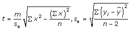
Information and hypothesis testing for slope.
When testing the slope M of the regression line for the population, you usually test that the slope is 0, or H0: M = 0. A slope of 0 indicates that there is no linear relationship between x and y. to perform the t-test for the slope of regression line and se is the standard error of estimate. Then, use the critical values found in a t-distribution table to make a decision whether to reject or fail to reject the null hypothesis. Alternatively, you can use technology to calculate the standardized test statistic as well as the corresponding P-value. If P ≤ α, then reject the null hypothesis. If P>α, then do not reject H0.
18. Construct the 95% confident interval for B and M, of the regression line y = Mx = B, for the population using the following inequalities and data.
B: b - E < B < b + E where E =
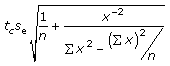
M: m - E < M < m + E where E =
|
x
|
y
|
x
|
y
|
|
2.3
|
222
|
1.4
|
183
|
|
1.7
|
179
|
1.6
|
180
|
|
1.9
|
217
|
2.1
|
181
|
|
2.5
|
244
|
2.1
|
209
|
19. The equation used to predict the total body weight (in pounds) of a female athlete at a certain school is y^= -116 + 3.161x1 + 1.56x2, where x1 is the female athlete's height (in inches) and x2is the female athlete's percent body fat. Use the multiply regression equation to predict the total body weight for a female athlete who is 63 inches tall and has 21% body fat.
The predicted total body weight for a female athlete who is 63 inches tall and has 21% body fat is pounds.
20. Use technology to find the multiple regression equation for the data shown in the table. Then answer the following.
a. What is the standard error estimate?
b. What is the coefficient of determination?
|
y
|
123.3
|
211.2
|
385.9
|
475.8
|
641.8
|
716.1
|
768.6
|
806.6
|
851.8
|
893.6
|
933.5
|
|
xi.
|
1.9
|
2.3
|
3.0
|
3.6
|
4.3
|
4.6
|
4.7
|
4.8
|
4.9
|
5.0
|
5.1
|
|
x2
|
13.9
|
17.7
|
21.9
|
25.9
|
32.1
|
37.9
|
39.0
|
39.4
|
40.1
|
41.9
|
42.1
|
21. Suppose a multiple regression has 7 independent variables. The coefficient of determination is found to be 0.958 based on a sample of 20 paired observations. After calculating r2adj. Compare this result with the one obtained using r2.