CLASSICAL PETRI NETS

 Petri nets, ever as Carl Adam Petri has proposed them in 1962 year, have formed a classical model of concurrency that non-determinism and control flow. Petri nets are bipartite graphs and recommend a mathematically and an elegant rigorous modelling framework for discrete event dynamical systems. Modelling via Petri nets is done employing Petri net objects in a top-down fashion. In order to solving the conflicts happening in the Petri net execution, real time high-level control systems are independently modelled and integrated along with the Petri net models.

Basic Definitions

In order to attain an in-depth understanding of Petri nets and its applications, we should first start a few fundamental definitions that are concerned to Petri nets.

Definition 1: The Classical Petri Net

A Petri net is defined as a four-tuple. (P, T, IN, OUT) here,

P = { p₁ , p₂ , ... , p_n }

T = {t₁ , t₂ , ... , t_n }

Above is a set of transitions.

P ∪ T ≠ Φ, P ∩ T = Φ

Here, P is a set of places, and

T is a set of transitions.

IN: (P × T) → N is an input function explain the arcs emanating from places to transitions.

OUT: (P × T) → N is an output function explains the arcs emanating from transitions to source.

By graphically, the places are shown by circles and transitions by vertical or horizontal bars. Places in a Petri net presentation normally model the condition or resources or state while the transitions are employed to depict the activities in a system. In order to generate a clear view we take up an easy example as shown below.

Illustration .1

We take up an illustration of a manufacturing system constituted of only a machine and processing a job. All part undergoes an operation upon the machine and after such the part is unloaded from the system and the machine is ready for a part's fresh piece to be processed. Following figure depicts the Petri net model of the manufacturing system discussed.

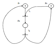
Figure: Petri Net Model of a Simple Manufacturing System Constituting of a Single Machine Processing a Job

                                 Table no.1: Interpretation of Places and Transitions as Shown in Petri Net of Figure

In the manufacturing illustration shown here we have the given:

P = { p₁ , p₂ , p₃}

T = {t₁ , t₂ }

The directed arcs shows the output and the input functions IN and OUT respectively such that,

IN (p₁, t₁) = 1

But,      IN (p3, t1) = 0

In the same way,

OUT (p3, t2) = 1

But,      OUT (p3, t1) = 0

Additionally, above Petri net has maximum arc weight as 1 hence can explain the above Petri net in a simpler notation employing a set A such as the Petri net is now explained as the 3-tuple (P, T, A)

Here A is,

A ⊆ (P × T ) ∪ (P × P)

Consider the Petri net above in Figure and determine the set A accordingly. By definition we contain the set A given by:

A =       {

 (p1, t1), (p2, t1), (p3, t2),

(t1, p3), (t2, p1), (t2, p2)

};

Definition 2: IP (t_j) and OP (t_j)

Moreover, for all transition t_j we have IP (t_j) which consequent to a set of all the places such as the arcs emanating from it end up on the transition t_j. Likewise, we have the OP or t_j that corresponds to a set of all the places such as the arcs emanating from it end up at the output places.

By using definition we have,

IP (t_j) = { p_i ∈ P : IN ( p_i , t_j ) ≠ 0}

OP (t_j) = { p_i ∈ P : OUT ( p_i , t_j ) ≠ 0}

Illustration 3

In above illustration 1 fined the IP (t₁) and OP (t₁)

Solution

IP (t₁) = {p₁, p₂}

OP (t₁) = {p₃}

Definition 3: IT (p_i) and OT (p_i)

For every place p_i we define IT (p_i) like a set of input transitions such as all the arcs emanating from those transitions end up on the place p_i. Likewise, we define OT (p_i) like the set of output transitions such as all the arcs emanating from pi end up at those transitions.

Hence by definition we have:

IT ( p_i ) = {t_j ∈ T : OUT ( p_i , t_j ) ≠ 0}

OT ( p_i ) = {t_j ∈ T : IN ( p_i , t_j ) ≠ 0}

Thus proved

(b) From definition 2 and definition 3 as given above we can easily visualize that:

OP (t₂) = {p₁, p₂}

IP (t₁) = {p₁, p₂}

Hence we can say that,

OP (t₂) = IP (t₁) = {p₁, p₂}

Thus proved

Definition 4: Marking of a Petri Net

A marking of a Petri net is a function M: P → N, here N is a set of natural numbers.

A marked Petri net is a Petri net along with an associated marking.

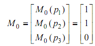
A marking of a Petri net is a vector (n × 1), here n stands for the number of places in the Petri net. Along with each place specific number of tokens are associated that are shown by dots. Mostly M₀ is utilized to represent the primary state of the Petri net. Usually the term state and marking are employed interchangeably.

Hence initial marking M₀ is defined as:

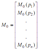
Illustration .6

In the Petri net represented in the figure of illustration.1 the initial marking is specified by the following vector as: