In the previous section we looked at the method of undetermined coefficients for getting a particular solution to

p (t) y′′ + q (t) y′ + r (t) y = g (t)    .....................(1)

and we observed that while it decreased things down to just an algebra problem, the algebra could become fairly messy. On the top of such undetermined coefficients will merely work for a fairly tiny class of functions.

The method of Variation of Parameters is a very general method which can be used in many more cases. Though, there are two drawbacks to the method. Firstly, the complementary solution is absolutely needed to do the problem. It is in contrast to the method of undetermined coefficients where this was advisable to contain the complementary solution on hand, although was not needed. Second, as we will notice, so as to complete the method we will be doing a couple of integrals and there is no guarantee as we will be capable to do the integrals. Therefore, while this will always be possible to write down a formula to find the particular solution, we may not be capable to actually get it if the integrals are too difficult or if we are not capable to find the complementary solution.

We're intended for derive the formula for variation of parameters. We'll start off through acknowledging as the complementary solution to (1) is

yc (t ) = c₁ y₁ (t ) + c₂ y₂ (t)

Remember also that it is the general solution to the homogeneous differential equation.

p (t ) y′′ + q (t ) y′ + r (t ) y = 0    ............. (2)

 As well as recall that so as to write down the complementary solution we know as y₁(t) and y2(t) are a fundamental set of solutions.

What we're going to do is notice if we can determine a pair of functions, u₁(t) and u₂(t) hence,

Y_P (t) = u₁(t) y₁(t ) + u₂(t ) y₂(t )

It will be a solution to (1). We have two unknowns now and so we'll require two equations eventually. One equation is simple. Our proposed solution should satisfy the differential equation, thus we'll get the first equation by plugging our proposed solution in (1). The second equation can arrive from a variety of places. We are going to determine our second equation simply through making an assumption as we will make our work easier. We'll say more regarding to this shortly.

Therefore, let's start. If we're going to plug our given solution in the differential equation we're going to require some derivatives hence let's get those. The first derivative is,

Y_P (t) = u'₁y₁ + u₁ y'₁ + u'₂ y₂ + u₂ y'₂

There is the assumption. Just to create the first derivative easier to deal along with we are going to suppose that whatever u₁(t) and u₂(t) are they will satisfy the subsequent.

u'₁ y₁ + u'₂ y₂ = 0   .........................(3)

Here's no motive ahead of time to believe that it can be done. Though, we will notice that it will work out. We simply create this assumption on the hope which it won't cause problems down the road and to create the first derivative simple so don't get excited regarding to it.

With this assumption the first derivative turns into,

Y'_P(t) = u'₁ y₁ + u'₂ y₂

The second derivative is after that,

Y''_P(t) = u'₁ y'₁ + u₁y''₁ +u'₂ y'₂ + u₂ y''₂

Plug the solution and its derivatives in (1).

p(t) (u'₁ y'₁ + u₁ y''₁+ u₂ y''₂) + q(t) (u₁ y'₁ + u₂ y'₂) + r(t) (u₁ y₁ + u₂ y₂) = g(t)

 Rearranging a little gives the subsequent,

p(t) (u'₁ y'₁ + u'₂ y'₂) + u₁(t) (p(t) y''₁ + q(t) y'₁ + r(t)y₁) + u₂(t) (p(t) y''₂ + q(t) y'₂ + r(t)y₂) = g(t)

Here, both y₁(t) and y₂(t) are solutions to (2) and therefore the second and third terms are zero. Acknowledging this and rearranging a little provides us,

p(t) (u'₁ y'₁ + u'₂ y'₂) + u₁(t)(0) + u₂(t)(0) = g(t)

 (u'₁ y'₁ + u'₂ y'₂) = (g(t))/(p(t))   ............................(4)

We've mostly got the two equations which we need. Before proceeding we're try to go back and create a further assumption. The previous equation, (4), is in fact the one that we want, however, so as to make things simpler for us we are going to suppose that the function p(t) = 1.

Conversely, we are going to go back and start working along with the differential equation,

y′′ + q (t) y′ + r (t) y = g (t)

If the coefficient of the second derivative isn't one divide this out hence it turns into a one. The formula which we're going to be getting will suppose this! Upon doing this the two equations which we need so solve for the unknown functions are

 u₁′ y₁ + u₂′ y₂ = 0   ....................(5)

u₁′ y₁′ + u₂′ y₂′ = g (t )    ...........(6)

Notice that in this system we know the two solutions and therefore the simply two unknowns there are u₁′ and u₂′.  Solving this system is in fact quite easy. Firstly, solve (5) for u₁′ and plug this in (6) and do several simplification.

u₁′ = - (u₂′ y₂/y₁)  ...................(7)

- (u₂′ y₂/y₁) y'₁ + u'₂ y'₂ = g(t)

u'₂(y'₂ - (y₂y'₁)/y₁) = g(t)

u'₂ =( y₁g(t))/( y₁ y'₂-y₂y'₁)   ..................(8)

Thus, we now have an expression for u₂′.  Plugging it in (7) will provide us an expression for u₁'.

u'₁ =- (( y₂g(t))/( y₁ y'₂-y₂y'₁)).......(9)

Then, let's notice that,

W(y₁y₂) = y₁y'₂ - y'₁y₂≠ 0

Recall that y₁(t) and y₂(t) are a fundamental set of solutions and thus we identify that the Wronskian won't be zero!

At last, all that we require to do is integrate (8) and (9) so as to determine what u₁(t) and u₂(t) are.  Doing this provides,

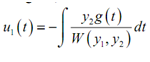
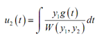
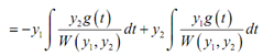
Thus, provided we can do these integrals, an exact solution to the differential equation is

Y_P(t) = y₁u₁ + y₂u₂

Therefore, let's summarize up what we've found here.