Reference no: EM131307193 , Length: word count:1500

1 Download and preprocess daily discharge data from USGS

Explore the National Water Information System (https://waterdata.usgs.gov/nwis) to find dis- charge gauges across the United States with long time series records. Search for sites with mean annual discharge exceeding 10 m3s-1. Be aware that USGS reports discharge in cfs (ft3s-1). "Self "-studying how to navigate on the NWIS site is part of the test.

Download discharge time series

Table 1:  Site attributes of the USGS station.

USGS Site:             04273500

Station Name:     Saranac river at Plattsburgh, NY Latitude:  44?40r54 N

Longitude:            73?28r16 W

HUC:                        02010006

Elevation:                47.47 m

Drainage Area:      1575 km2

(Figure 1) for a station of your choice and import the downloaded data into R. Please note that USGS reports from several thousands dis- charge gauges so an excessive number of students accidentally picking the same site will look suspicious. The discharge records can be saved as an ASCII text file, which will have sev-eral lines of headers followed by fixed with tabular format. You can use a regular text editor to remove the header lines and keep only the one with column names followed by the data. Alter- natively, you can specify the number of lines to be skipped in the (read.table(), read.csv() or read.ftable()) R functions. These functions will return the content of the discharge data file as dataframe, which can be viewed as structured vector, where the number of vector elements correspond to individual daily discharge observation and the record structure contains the columns from the loaded data. The members of the structures can be accessed via the $ sign separator.

The data series in the presented example had missing data as blank or marked by text like "ice " causing the read.csv() function to read the col- umn as "factor". The factor data type encodes the values as an inte- ger index and a corresponding text string as level. Be aware that the as.numeric() function for factor data types returns the index value, while as.character() returns the level as text string (which contains the actual reported values), therefore one needs to convert the factor into character first and convert the re-sulting text string into numeric variables in a second step.

Collect the corresponding station attribute data for the selected site (Table 1). Convert the reported elevation and drainage area to metric units (m above sea level and km2) along with the downloaded discharge time series (from cfs to m3s-1).

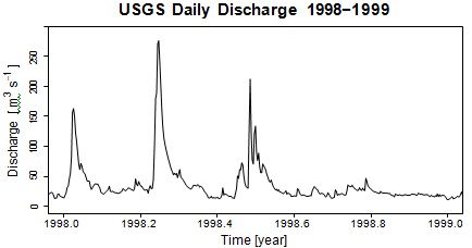
Plot the downloaded daily discharge time series for two or three years period of your choice (Figure 1). For plotting the daily data for multiple years, you might need a new date column that represents time in decimal years (that is expressing the day and month as the fraction of the year. The decimal date() function from the lubridate package is readily available to perform this task.

2 Aggregate the daily data and compute relevant statistics

Compute the annual average, the standard deviation, the maximum and the minimum of the daily dis- charge for each year. One of the possible means to aggregate the daily discharge data imported into R as dataframe is the R func- tions provided by the dplyr pack- age. You will need to split the date field in the dataframe using the substring() function into year, month and day columns. Using the group by() function the daily data can be grouped by the year column from the discharge data dataframe and the summarize() function can aggregate the daily discharge values by mean() - mean/average, sd() - standard deviation, max() - maximum, min() - minimum. Plot the resulting annual dis- charge time series of mean, ± standard deviation around the mean, maximum and minimum dis- charge of your selected site (Figure 2). You will need to pass valid daily discharge values that you can extract from your discharge data vector using the na.omit() function.

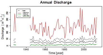
Figure 2: Annual discharge time series of the Saranac River at Plattsburgh, NY (USGS Gauge #04273500).

Compute the mean, the standard deviation, the maximum and the min- imum of the daily discharge for each day (from January 1st to Decem- ber 31st) during your observational records. This step will require cal- culating the day of the year from the observation date. Using the strptime() function you can convert the date string from the discharge records dataframe into POSIX stan- dard date that the strftime() func- tion can recognize and convert to day of the year specifying j". Plot the resulting daily discharge cli- matology time series (Figure 3).

Daily mean/average, minimum and maximum dis- charge at the Saranac River at Plattsburgh, NY (USGS Gauge #04273500) discharge gauging station.

3 Fitting theoretical distributions functions to daily discharge data

Fit theoretical distributions (normal, lognormal, gamma and exponential ) to the daily discharge values. Use the fitdistr() function from MASS package that will apply maximum-likelihood methord to find the relevant parameters. The fitdistr() will return a dataframe where the
<dataframe-of-your-choice>$estimate[] member will hold the parameter values. The param- eters themselves can be accessed as <dataframe-of-your-choice>$estimate['<parameter>'] where the <parameter> will vary as a function of the theoretical distribution functions. Create

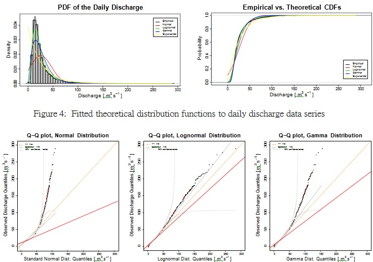
Figure 5: Q-Q plots of the empirical and theoretical probability distributions of the daily discharge values.

a vector of sorted unique valid discharge values of your daily time series. Use the sort() and unique() functions on the valid discharge values obtained from na.omit() function.

Plot the theoretical probability density functions against the histogram of the daily discharge values using the hist() function and empirical density obtained from the density() function. You will need the full time series (without the nodata values). The theoretical density function can be computed for the sorted unique values by applying the appropriate PDF and CDF functions (e.g. dnorm() and pnorm() for normal distribution (Figure 4).

A Quantile-Quantile (Q-Q) plot is a scatter plot comparing the fitted and empirical distributions in terms of the dimensional values of the variable (i.e., empirical quantiles). It is a graphical technique for determining if a data set come from a known population. In this plot on the y-axis we have empirical quantiles on the x - axis we have the ones got by the theoretical model. Produce Q-Q plots for normal, lognormal and gamma distributions. Use the qqplot() function from the extRemes package (Figure 5).

4 Kolmogorov-Smirnov Goodness-of-fit test

The Kolmogorov-Smirnov test is used to decide if a sample comes from a population with a specific distribution. It is based on a comparison between the empirical distribution function (ECDF) and the theoretical one.

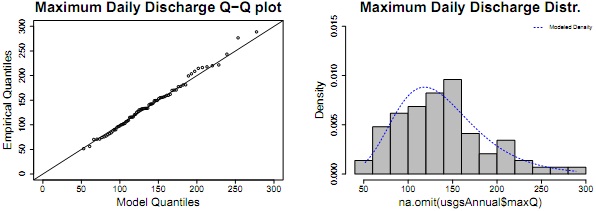
Figure 6: Q-Q plot of the fitted GEV distribution and observed maximum daily dischareg and the histogram along with the GEV probability distribution

Use the ks.test() function from the stats package (normally loaded by default) with the unique sorted data vector and the corresponding CDF vector computed in the previous problem to test if any of the theoretical distribution functions (normal, lognormal, gamma or exponential have more the p = 5 % significance.

5 Extreme value distribution

Fit general extreme value distribution (GEV) to the maximum daily discharge data series using the fevd() function from the extRemes package. Pass the maximum daily discharge data series to the fevd() function after ex- cluding nodata values (na.omit()) and use the type="GEV" option. This will return a fevd list object class that can be used in other extreme value related functions. For instance, you should retrieve the parameters of the GEV distributions along with their 95 % using the ci() function with type=parameter option (Table 2).

Table 2: GEV parameters with 95 % confidence bounds

	lower CI	Estimate	upper CI
location	105.32	116.20	127.08
scale	33.84	41.73	49.62
shape	-0.23	-0.05	0.13

You should also compute the maximum daily discharge associated with different return periods. The return.level() function is readily available for this task. Compute return periods for 5, 10, 50, 100 and 500 years along with their confidence bounds by passing the do.ci=TRUE option (Table 3). You can perform this task by a single call to the return.level() funciton by passing a vector of the requested return periods.

The extRemes package adds a series of methods to the plot() function to simplify pro- ducing plots from the fevd list object class re- turned by the fevd() function. Create a Q-Q plot and the histogram of the maximum daily discharge along with GEV density function. You can create these plots by simply passing the fevd list object to the plot() function (Figure 6).

Table 3: Maximum daily discharge (m3s-1) return periods with 95 % confidence bounds

Return Period	lower CI	Estimate	upper CI
5-year	160.38	176.48	192.58
10-year	183.56	204.97	226.38
50-year	217.87	264.00	310.13
100-year	225.90	287.51	349.13
500-year	232.12	338.78	445.45

6 Final Report

Summarize your work in a professional looking report including figures and tables. The report should include a brief description of the site you picked possibly with a map of the site location using Google Map (a screen shot is sufficient) and a discussion of the computation you carried out. The proper means of creating figures is to use the postscript(), pdf(), bmp, png() or tiff() graphical device functions that can be called before the plot() command and subsequent calls to other drawing commands (e.g. points or line()). Once the plot is complete, you will need to call dev.off() function to finish the plot and ensure that R writes all the graphical objects into file. These graphical device function will not only allow producing graphics as files that can be inserted into text documents, but enables controling the image size and resolution that is necessary for producing publication quality images.

Make sure that your plots have proper title, axis labels and legends (you can use the legend() function to draw legends). The plot() function attempts to put reasonable labels and titles onto each figure, but most of the time those lables are imperfect. Make sure that the figures are labeled properly by specifying the main, xlab, ylab options. Include appropriate units in the axis labels with proper superscripts.

The default values of the font sizes are not particularly pretty. Explore the relevant plotting options to change the look of your figures. The overall look of your report will be a factor in your final grade on this test.

The R script of your work should be part of your report as Appendix and the report has to be in PDF format.