Conduct a granger causality analysis

Assignment Help Applied Statistics

Reference no: EM131273836

Problem 1- Time Series Analysis

For this assignment you will fit a series of frequentist VAR models. You will need to closely consult the Brandt and Williams (2007), and Brandt and Freeman (2006) readings for the VAR. analyses. These will be especially useful for interpreting the results of your analyses.

The data file is located on the course website in a Stata file called polity.dta. It contains three monthly time series from 1978-2004: Michigan Index of Consumer Sentiment (mics),

U.S. Presidential Approval (approve), and Macropartisanship (mp).

The R packages MSBVAR, and vars will be most useful for this assignment.

The following initial R code will get you started reading in the data and setting up the time series:

> library(foreign)
> d <- read.dta("polity.dta")
> attach(d)
> Y <- ts(cbind(mics, approve, mp), start=c(1978,1), freq=12)
> colnames(Y) <- c("Consumer Sentiment", "Approval", "Macropartisanship")
> detach(d)

In this first part of the assignment you will fit and interpret a frequentist VAR model for the data. Perform the following analysis and be sure to fully interpret and report your results (i.e., don't just tell us the lag length for the VAR is p. Explain how you came to this conclusion and other results).

1. Test the series to determine the lag length for a VAR model.
> # Load the libraries -- do the urca library for the unit root tests.
> library(MSBVAR)
> # Lag length testing
> lag.choice <- var.lag.specification(Y)
> print(lag.choice)

$ldets
Lags Log-Det Chi^2 p-value [1,] 20 6.493766 7.871991 5.470963e-01
[2,] 19 6.526161 10.097943 3.426146e-01

[3,] 18 6.567210 12.959778 1.644347e-01
[4,] 17 6.619257 10.034583 3.476928e-01
[5,] 16 6.659077 6.984073 6.387777e-01
[6,] 15 6.686465 7.596517 5.752617e-01
[7,] 14 6.715909 13.851149 1.277195e-01
[8,] 13 6.768979 13.725604 1.324263e-01
[9,] 12 6.820970 5.745679 7.650773e-01
[10,] 11 6.842489 12.573879 1.828544e-01
[11,] 10 6.889059 7.858298 5.484872e-01
[12,] 9 6.917844 9.522480 3.905059e-01
[13,] 8 6.952346 9.772719 3.691964e-01
[14,] 7 6.987373 12.084817 2.085698e-01
[15,] 6 7.030227 12.000439 2.132846e-01
[16,] 5 7.072334 10.785072 2.907294e-01
[17,] 4 7.109782 17.254018 4.488354e-02
[18,] 3 7.169075 10.867864 2.848751e-01
[19,] 2 7.206040 52.566123 3.532100e-08
[20,] 1 7.383030 0.000000 0.000000e+00

$results

[1,] Lags
1 AIC 7.461978 BIC 7.608703 HQ 7.520671
[2,] 2 7.344198 7.600966 7.446911
[3,] 3 7.366443 7.733255 7.513176
[4,] 4 7.366361 7.843217 7.557115
[5,] 5 7.388124 7.975023 7.622897
[6,] 6 7.405227 8.102170 7.684021
[7,] 7 7.421584 8.228570 7.744397
[8,] 8 7.445767 8.362797 7.812600
[9,] 9 7.470476 8.497549 7.881329
[10,] 10 7.500901 8.638018 7.955775
[11,] 11 7.513542 8.760702 8.012435
[12,] 12 7.551233 8.908437 8.094146
[13,] 13 7.558453 9.025700 8.145386
[14,] 14 7.564593 9.141885 8.195547
[15,] 15 7.594360 9.281695 8.269334
[16,] 16 7.626182 9.423561 8.345176
[17,] 17 7.645573 9.552995 8.408586
[18,] 18 7.652736 9.670202 8.459770
[19,] 19 7.670898 9.798407 8.521952
[20,] 20 7.697714 9.935266 8.592787

attr(,"class")
[1] "var.lag.specification"

> # Set the lag length to p. Here we choose 4 because the 4th lag is
> # significant. Were better off over-fitting a VAR on lag length,
> # especially if we think there is non-stationarity.
> p <- 4

2. Using the lag length you select in the previous step, conduct a Granger causality analysis. Report the results in a table.

> gc.results <- granger.test(Y, p)
> print(gc.results)

	F-statistic	p-value
Approval -> Consumer Sentiment	1.2133144	0.30505798
Macropartisanship -> Consumer Sentiment	0.7949978	0.52914198
Consumer Sentiment -> Approval	1.3809165	0.24036859
Macropartisanship -> Approval	1.3961989	0.23511102
Consumer Sentiment -> Macropartisanship	0.9321858	0.44544747
Approval -> Macropartisanship	2.3274438	0.05623189

3. Fit a reduced form VAR model for these data.
> rf.var <- reduced.form.var(Y, p)

4. Generate impulse response functions (IRFs) for the reduced form model you fit in the last step. Given that the data are monthly and this is American political data, you will need to make a choice about what time horizon to use.
> # Here we will look at 48 months of responses.
> rf.irfs <- irf(rf.var, nsteps=48)
> # Now plot the responses
> plot(rf.irfs, varnames=colnames(Y))

[,1] [,2] [,3]
[1,] -0.5957623 -0.5043421 -0.4000981
[2,] 3.6586221 4.1378754 2.2821363

The results of this step are show in Figure 1.

5. Now redo the previous step and generate a set of Monte Carlo error bands for the impulse responses using 10000 samples.
> rf.mc.irfs <- mc.irf(rf.var, nsteps=48, draws=10000)

Monte Carlo IRF Iteration = 1000 Monte Carlo IRF Iteration = 2000 Monte Carlo IRF Iteration = 3000 Monte Carlo IRF Iteration = 4000

Monte Carlo IRF Iteration = 5000 Monte Carlo IRF Iteration = 6000 Monte Carlo IRF Iteration = 7000 Monte Carlo IRF Iteration = 8000 Monte Carlo IRF Iteration = 9000 Monte Carlo IRF Iteration = 10000

> plot(rf.mc.irfs, method="Sims-Zha2", component=1, probs=c(0.05, 0.95),
+ varnames=colnames(Y))

The results of this step are show in Figure 2.

6. Now comment on what dynamic factors affect presidential approval and macroparti- sanship. That is, interpret the impulse responses you generated.

You will find that the sentiment measures drive approval and there are weak responses in the aggregate partisanship measures.

[,1] [,2] [,3]
[1,] -0.5957623 -0.5043421 -0.4000981
[2,] 3.6586221 4.1378754 2.2821363

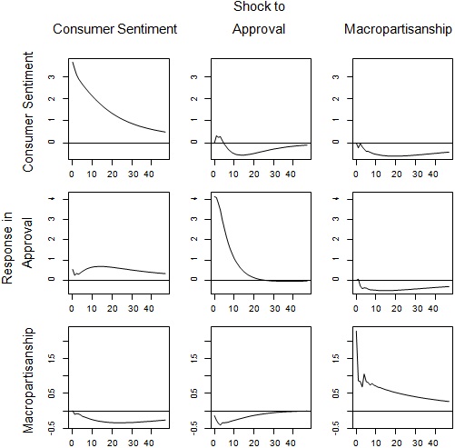
Figure 1: Impulse responses for the reduced form VAR for consumer sentiment, approval and macropartisanship. Rows correspond to equations, columns to the shocks.

Monte Carlo IRF Iteration = 1000
Monte Carlo IRF Iteration = 2000
Monte Carlo IRF Iteration = 3000
Monte Carlo IRF Iteration = 4000
Monte Carlo IRF Iteration = 5000
Monte Carlo IRF Iteration = 6000
Monte Carlo IRF Iteration = 7000
Monte Carlo IRF Iteration = 8000
Monte Carlo IRF Iteration = 9000
Monte Carlo IRF Iteration = 10000

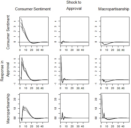
Figure 2: Impulse responses for the reduced form VAR for consumer sentiment, approval and macropartisanship. Rows correspond to equations, columns to the shocks. Error bands are likeihood-based 90% credible intervals.

Problem 2 - Time Series Analysis

For this assignment you will compare a series of frequentist and Bayesian VAR models. You will need to closely consult the Brandt and Williams (2007), and Brandt and Freeman (2006) readings for the VAR/BVAR analyses. These will be especially useful for interpreting the results of your analyses.

The data file is located on the course website in a Stata file called polity.dta. It contains three monthly time series from 1978-2004: Michigan Index of Consumer Sentiment (mics),

U.S. Presidential Approval (approve), and Macropartisanship (mp).

The R packages MSBVAR, and urca will be most useful for this assignment. You will need MSBVAR for the Bayesian part and to do the different error bands-vars cannot estimate them.

The following initial R code will get you started reading in the data and setting up the time series:

Part 1

In this first part of the assignment you will fit and interpret a frequentist VAR model for the data (so this parallel's the last assignment). Perform the following analysis and be sure to fully interpret and report your results (i.e., don't just tell us the lag length for the VAR is p.

Explain how you came to this conclusion and other results).

1. Test the series to determine the lag length for a VAR model. Also check for the presence of unit roots.

2. Fit a reduced form VAR model for these data.

3. Generate impulse response functions (IRFs) for the reduced form model you fit in the last step. Given that the data are monthly and this is American political data, you will need to make a choice about what time horizon to use (hint 24 or 48 months).

4. Now redo the previous step and generate a set of Monte Carlo error bands for the impulse responses.

Part 2

In this part of the analysis you will fit a series of Bayesian VAR models for the data in Part 1.

1. Consider an initial BVAR model with the Sims-Zha prior. Use the following for the initial hyperparameter values: λ0 = 0.8, λ1 = 0.1, λ3 = 1, λ4 = 0.1, λ5 = 0, µ5 = 3, µ6 = 3.

2. Systematically evaluate different hyperparameters / priors and the sensitivity of the results to your choices. Use the SZ.prior.evaluation function to compare the priors.

3. Fit a final BVAR based on your sensitivity analysis and report the results via IRFs and comment on how these differ from the frequentist ones.

Attachment:- polity.rar

Reference no: EM131273836

Questions Cloud

How can you enhance your voice mail presence : What steps will you take to enhance your telephone presence? How can you enhance your voice mail presence? What steps will you take to enhance your e-mail communication?

Differences in international marketing and global marketing : We currently operate in a business environment driven by technology and trade agreements that provide companies access to multiple environments. The marketing discipline has been forced to evolve and adapt to this environment. Companies still need to..

Duration of bond and why is knowing bond duration useful : A bond with a par value of $1,000 and a 6% semi-annual coupon rate has 9 years to maturity. Assuming it is priced to yield 8%, compounded semi-annually, what is the market price of the bond, to the nearest dollar? Discuss some of the major social med..

Experiencing an inflationary gap and the government : If the economy is experiencing an inflationary gap and the government wants to accelerate the adjustment to the long-run equilibrium through fiscal policy, it should:

Conduct a granger causality analysis : Fit a final BVAR based on your sensitivity analysis and report the results via IRFs and comment on how these differ from the frequentist ones - Conduct a Granger causality analysis

How you will propose technology be implemented : Discuss how technologies or information systems have contributed to the problem. Discuss how you will propose technology be implemented into the solution.

According to the online lecture, what do most jews feel abo : What does it mean to say, in Judaism, that God is both "transcendent" and "immanent"?

Decide whether or not there was a contract for the purchase : Decide whether or not there was a contract for the purchase of the automobile. Identify the facts from the scenario which support your decision on whether or not a contract exists for the purchase of the automobile.

What are pros and cons of outsourcing and offshoring : Explain the limits on the types of products and services a commercial bank can offer. What are pros and cons of outsourcing and offshoring? Should we curtail outsourcing and offshoring to protect jobs? Discuss with an example a situation where a cour..

User Account

All Pages